
Semantic Segmentation and Model Fitting for Triangulated Surfaces
using Random Jumps and Graph Cuts
Tilman Wekel and Olaf Hellwich
Computer Vision Group, TU-Berlin, Berlin, Germany
Keywords:
Segmentation, Multi Label, RANSAC, Graph Cut, Reverse Engineering, Random jumps.
Abstract:
Recent advances in 3D reconstruction allows to acquire highly detailed geometry from a set of images. The
outcome of vision-based reconstruction methods is often oversampled, noisy, and without any higher-level
information. Further processing such as object recognition, physical measurement, urban modeling, or ren-
dering requires more advanced representations such as computer-aided design (CAD) models. In this paper,
we present a global approach that simultaneously decomposes a triangulated surface into meaningful seg-
ments and fits a set of bounded geometric primitives. Using the theory of Markov chain Monte Carlo methods
(MCMC), a random process is derived to find the solution that most likely explains the measured data. A
data-driven approach based on the random sample consensus (RANSAC) paradigm is designed to guide the
optimization process with respect to efficiency and robustness. It is shown, that graph cuts allow to incor-
porate model complexity and spatial regularization into the MCMC process. The algorithm has successfully
been implemented and tested on various examples.
1 INTRODUCTION
The reverse engineering of CAD models based on tri-
angulated surfaces definitely belongs to the most im-
portant fields of 3D computer vision. The main chal-
lenge is to find a valid decomposition of the surface
which allows to fit a set of geometric models. This
is a typical chicken-and-egg problem. Many related
algorithms, however, try to tackle this problem by ap-
plying a set of sequential processing steps. In this
paper, we argue that the high presence of noise on the
one hand, and the bidirectional dependencies of these
steps on the other hand, require a global approach to
find an optimal solution. The proposed processing
flow is motivated in Figure 1. Especially mechanical
objects can be described as a composition of bounded
geometric primitives (a). Towards CAD-based appli-
cations, we aim at reconstructing a geometric repre-
sentation from a noisy triangulated surface (b). Si-
multaneously, the surface is decomposed into mean-
ingful segments (c), where each segment corresponds
to a component of the object. The object as well as
the labeling of the vertices define a ”world state”.
From a Bayesian perspective, we want to find the
state which most likely explains the observation. The
resulting optimization problem is defined in a high-
dimensional and non-continuous domain. The jump-
diffusion framework seems to be particularly suited
for these complex problems. It allows to optimize en-
ergy functions which are defined in a complex space
that includes several sub domains of different dimen-
sions. Secondly, it can escape from local minima.
1.1 Contributions
This paper contains several new contributions. An
MCMC process is designed for the purpose of mesh
processing. The semantic segmentation is formulated
as an inference problem based on a triangulated sur-
face. Compared to related algorithms, we incorporate
model complexity and spatial regularization into the
random-jumps process. A crucial aspect of MCMC
methods is the computation of the proposal probabil-
ities. We show, that RANSAC allows to compute a
non-uniform distribution that balances efficiency and
robustness against local minima.
1.2 Overview
The remaining part of the paper is structured as fol-
lows. A brief overview of related approaches is given
in Section 2. In Section 3, we formulate the task as
an inference problem. An energy function is derived
to evaluate the likelihood of the current state. In Sec-
241
Wekel T. and Hellwich O..
Semantic Segmentation and Model Fitting for Triangulated Surfaces using Random Jumps and Graph Cuts.
DOI: 10.5220/0005265102410250
In Proceedings of the 10th International Conference on Computer Vision Theory and Applications (VISAPP-2015), pages 241-250
ISBN: 978-989-758-091-8
Copyright
c
2015 SCITEPRESS (Science and Technology Publications, Lda.)
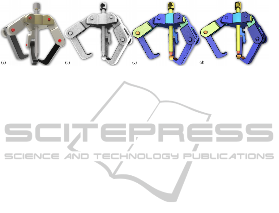
Figure 1: Schematic illustration of the reverse-engineering problem. An object is given in (a). The object is measured by
a vision- or laser-based reconstruction tool chain which results in a noisy triangulated surface (b). The problem is now to
recover the original object based on the measurement and some general prior knowledge. Especially man-made geometry can
be described by a set of bounded geometric primitives. The proposed algorithm robustly decomposes the triangulated surface
into meaningful segments (c) and recovers a set of components accordingly (d).
tion 4, we briefly introduce geometric primitives and
define the corresponding cost functions. Finally, we
design a MCMC process in Section 5 in order to ro-
bustly minimize the energy function. The resulting
algorithm has been successfully implemented and an
evaluation can be found in Section 6. The paper con-
cludes with Section 7.
2 RELATED WORK
The presented approach is related to a broad field
of algorithms which can roughly be subdivided into
multi-model fitting problems, mesh segmentation and
classification. In the following, an overview of related
work is given.
2.1 Mesh Segmentation and
Classification
There has been a lot of attention to the problem of
mesh segmentation. Many segmentation algorithms
are inspired by classical machine learning methods,
such as hierarchical clustering, k means, or mean
shift. Based on the fitting of three different geometric
primitives, Attene et al. propose a fast greedy method
that segments a given mesh by an iterative cluster-
ing scheme (Attene et al., 2006). Another impor-
tant group of algorithms follows the k-means strategy.
Cohen-Steiner et al. present an algorithm referred to
as variational shape approximation that is based on k
means (Cohen-Steiner et al., 2004). The partition step
is realized by a modified region growing scheme that
assures connected segments. Several other authors
propose modified or extended versions of the varia-
tional approach (Wu Leif Kobbelt, 2005)(Yan et al.,
2012). The most important problems of variational
methods are a suitable initialization and the adequate
choice of the number of clusters.
Especially suited for man-made geometry,
feature-based algorithms achieve an implicit seg-
mentation by detecting the blending regions. These
algorithms do not explicitly fit geometric models
(V
´
arady et al., 2007)(Mangan and Whitaker, 1999).
A (semantic) segmentation can also be achieved
by designing a classification problem, where each
vertex is assigned with a label which can have a
semantic meaning. This motivates to use methods
like Markov random fields or graph cuts. The spatial
regularization allow to achieve smoother boundaries
than variational or hierarchical methods. However,
the set of classes is fixed and need to be known
a priori. Related algorithms are often designed to
learn and apply a natural segmentation based on
large datasets of models such as animals, humans
or furniture(Longjiang et al., 2013)(Lavou
´
e and
Wolf, 2008)(Lai et al., 2008). They decompose
objects with respect to topology or the minima rule
which is mainly suited for organic shapes such as
humans or animals. Some approaches require a set of
similar training models which is often not available
in reverse-engineering scenarios (Kalogerakis et al.,
2010)(Benhabiles et al., 2011)(Lv et al., 2012).
2.2 Multi-model Fitting Problems
The challenge described in this paper is clearly related
to the class of multi-model fitting problems. Recently
there has been a lot of attention to this field. Roughly
summarized, there are three different approaches to
the fitting of multiple models.
2.2.1 Random Sample Consensus
First, RANSAC is a well-known strategy to esti-
mate model parameters in presence of a high num-
ber of outliers. In each iteration, a model candidate is
parametrized, based on a minimal set that is randomly
drawn from the input data. Each candidate is scored
VISAPP2015-InternationalConferenceonComputerVisionTheoryandApplications
242

by the number of inliers that are sufficiently explained
by the model. Schnabel et al. propose an efficient ap-
proach where RANSAC is used to extract primitive
shapes from a noisy point cloud in an iterative man-
ner. The result significantly depends on a set of pa-
rameters that are required to detect the inliers in the
sampling procedure (Schnabel et al., 2007). Papazov
et al. use a RANSAC-like strategy for the recognition
of high-level objects in scattered environments (Papa-
zov and Burschka, 2011). The greedy nature of multi-
RANSAC algorithms does not guarantee a global op-
timum. Li et al. uses RANSAC to globally fit a set
of primitives with respect to alignment constraints (Li
et al., 2011). There approach makes strong assump-
tions on the geometry of the object which is not al-
ways given.
2.2.2 Multi Labeling
Secondly, multi-model fitting can be solved by graph-
ical models such as MRFs or graph cuts. Delong et
al. have extended the α-expansion algorithm for in-
corporating label costs. The additional term in the
optimization function allows to minimize the number
of used classes or models explaining the data (De-
long et al., 2010). Based on multi-label optimization,
Isack and Boykov introduce an algorithm referred to
as PEaRL which iterates a two-step procedure (Isack
and Boykov, 2012). Given a set of geometric models,
the algorithm of Delong et al. is used to compute a la-
beling which incorporates label costs and spatial reg-
ularization. In the second step, the set of all models is
reconfigured by inserting new models, deleting obso-
lete models, or updating their parameters. The work
of Woodford et al. introduces a new type of contrac-
tion move for the optimization of multi-model fitting
problems (Woodford et al., 2012). The drawback of
these methods is that the update of the model config-
uration is deterministic and thus they cannot escape
from local minima.
2.2.3 Random Jumps
A third powerful and very general framework for
multi-model fitting is given by random jumps. Tu and
Zhu proposed an image segmentation approach based
on random jumps (Tu and Zhu, 2002). The image
is assumed to be a composition of a set of heteroge-
neous models that allow to describe typical regions
such as clutter, texture, or shading. The global en-
ergy function takes data costs and boundary smooth-
ness into account. As one of the key contributions,
they use data-driven techniques such as expectation
maximization or mean shift to compute new propos-
als and their corresponding probabilities. Han et al.
use a very similar framework to segment range images
based on geometric models (Han et al., 2004). Image
regions which cannot be fitted by any of these models
are described by a cluttered type which is a 3D his-
togram. Larfarge et al. use geometric primitives and
the MCMC framework for the reconstruction of so-
called hybrid models from a set of images and known
camera poses (Lafarge et al., 2013). Similar to Hang
et al., a hybrid model can either be a primitive or an
arbitrary shape which is represented by a triangular
mesh. The data term in the energy function enforces
photo consistency which measures the error between
the image projections of two cameras on a geometric
primitive. Model complexity as well as spatial reg-
ularization in the labeling of the mesh is not consid-
ered.
3 STOCHASTIC PROBLEM
FORMULATION
Consider a polyhedral surface S = {V, E, T}, which
consists of vertices V, edges E, and triangles T. S
is assumed to be a measurement (observation) of an
object O. The hidden world state is defined as:
Φ = {O, X }, |X | = |V| (1)
where Φ is the model O itself and the labeling X
which explicitly assigns a component of O to each
vertex on S. O is decomposed into K components:
O = {K, {M
k
, A}, k = [0, .. . , K]} , (2)
where a component M
k
= {r
k
, ∂
k
, θ
k
} is given by the
type of the underlying geometric primitive r
k
, a pa-
rameter vector θ
k
, and a boundary ∂
k
. Geometric
primitives are represented by implicit equations that
allow to efficiently compute distances or projections
(Schnabel et al., 2007). A is introduced as a default
model. From a classification perspective, A can also
be seen as an ”unassigned”-class that represents all
vertices which cannot be explained by any other class
in O. All components of O are associated with a label
l ∈ L:
L := {l
k
M
| k ∈ [0, . . . , K] , l
A
} , (3)
where l is the k-th unit vector. The labeling of the
vertices l → x implies a semantic segmentation on S,
S = {S
0
, . . . , S
K
, S
A
}, where S
k
corresponds to the set
of all vertices which are being labeled with l
k
. ∂
k
is
the boundary of the corresponding segment on S, ∂
k
=
∂S
k
. Finally, the overall problem is to find a world
state Φ
∗
that most likely explains a given observation,
S:
Φ
∗
= arg max
Φ∈Ω
p(Φ |S) . (4)
SemanticSegmentationandModelFittingforTriangulatedSurfacesusingRandomJumpsandGraphCuts
243

Figure 2: Effect of the prior term for the Grabber model.
The result in (a) is based on data cost only and 200 initial
shape candidates. The result of the MCMC process with a
low, non-zero prior can be seen in (b). If the regularization
parameters are set to higher values, the algorithm produces
a smaller number of segments and smoother boundaries, as
it can be seen in (c).
p(Φ|S) can be decomposed into prior and likelihood:
p(Φ|S) ∝ p(S|Φ)p(Φ) . (5)
For the sake of simplicity, the optimization problem
in Equation 5 is transferred to the log-probability do-
main:
Φ
∗
= arg min
Φ∈Ω
U(Φ, S) = U
D
(Φ, S) +U
M
(Φ) . (6)
U
D
(Φ, S) corresponds to the likelihood in Equation
5 and is referred to as data term in the optimization
community. U
M
(Φ) represents prior knowledge about
the spatial regularity and the model complexity of Φ.
3.1 Prior Distribution
As soon as assumptions or knowledge about the de-
manded model O is available, the prior distribution is
non uniform and allows to enforce specific properties
on Φ. The complexity of O is given by the complexity
of the models M
k
:
U
M
(O) =
K
∑
k=1
|M
k
| , M
k
∈ O , (7)
where |M
k
| represents the complexity cost for each
type of model. As specified in Table 4, we prefer
simple over more complex models. U
M
(O) is also
referred to as label cost term. Each vertex of S is as-
signed to a class and the set of all vertices implies
the boundary of the corresponding surface patch ∂
k
.
The label-based representation allows to minimize ∂
k
based on α-expansion (Delong et al., 2010):
U
∂
(X ) =
∑
(i, j)∈N
T
φ(x
i
, x
j
) , x
i
, x
j
∈ X , (8)
where φ(x
i
, x
j
) penalizes adjacent sites with different
labels. The overall term is then:
U
M
(Φ) = αU
M
(O) + βU
∂
(X ) . (9)
The strength of the regularization as well as of the
model-complexity term is controlled by α and β re-
spectively. If both values are set to zero, each ver-
tex is simply assigned to the closest component of
O, as it can be seen in Figure 2(a). The label costs
eliminate redundant components, while the smooth-
ness term enforces straight boundaries. The effect is
shown in (b). If the values for α and β are increased
further, the segmentation captures only the most im-
portant features, as it is seen in (c).
3.2 Likelihood
The likelihood term U
D
quantifies how well the state
Φ fits the observation S:
U
D
(Φ, S) =
∑
x
i
∈X ,v
i
∈S
< u(v
i
, O), x
i
> . (10)
u(v
i
, O) is a vectorial function, where the k-th entry
of u contains the cost for assigning l
k
→ x
i
, given the
observation v
i
∈ S. According to Equation 3, x
i
is
represented as a unit vector. The energy contribution
of each site can then be written as a scalar product of
u(v
i
, O) and x
i
.
4 GEOMETRIC MODELS
A component M
k
is given by the underlying geomet-
ric primitive which is fully defined by its type r and
its parameter vector θ
k
. For all considered geometric
models an orthogonal projection on M can be com-
puted for a given point: Π
θ
(·). The distance of a ver-
tex v
i
and a geometric primitive θ is defined as:
L
e
(v
i
, θ) = kp
i
− Π
θ
(p
i
)k , (11)
where a vertex is represented by its point p
i
. Π
θ
(q
i
) is
the projection of p
i
on the surface of θ. A component
M
k
has a likelihood which is assumed to be:
φ(v
i
, M
k
) =
L
e
(v
i
, θ
k
), if p
i
∈ N
ε
(M
k
)
∞, otherwise.
(12)
φ(v
i
, M
k
) has infinite cost if v
i
is not in the envi-
ronment of the component N
ε
(M
k
), which is defined
later. The overall cost vector for assigning v to each
model in O is:
u(v, O) =
(φ(v, M
1
), . . . , φ(v, M
K
))
T
c
A
. (13)
For a given vertex v, A is the preferred label if no
other component yields cost values lower than c
A
. In
practice, c
A
only needs to be set to a sufficiently large
number. This encourages the MCMC process to insert
models.
VISAPP2015-InternationalConferenceonComputerVisionTheoryandApplications
244
4.1 Bounded Geometric Primitives
Assume that a geometric primitive θ
k
∈ M
k
is given
which fits a subset of the triangulated surface S ac-
cording to Equation 12. Intuitively speaking, the like-
lihood for assigning a vertex v ∈ S to M
k
should de-
pend on the distance of v to θ
k
according to Equation
11. This is illustrated by the blue shading in Figure
3. However, geometric primitives are models with
infinite extend and a boundary is not explicitly rep-
resented in L
e
. This leads to many small clusters of
vertices which are assigned to θ
k
, as shown in Figure
3. We use the topology of S to recover the bound-
ary ∂M
k
on S. A function is defined, that indicates
all vertices which are spatially close to the geometric
primitive:
b(v, θ
k
) =
1, if L
e
(v, θ
k
) ≤ e
ε
0, otherwise.
. (14)
b(v, θ
k
) implies a partition of the surface into con-
nected components:
S = {S
b=1
M
k
, S
b=0
M
k
} . (15)
Moreover,
ˆ
S
b=1
M
is defined to be the largest connected
component in S
b=1
M
k
. The local environment of a model
is then defined as the subset of segments in S
b=1
M
k
which are bigger than a predefined threshold c
s
|
ˆ
S
b=1
M
k
|:
N
ε
(M
k
) = {∀S ∈ S
b=1
M
k
: |S| ≥ c
s
|
ˆ
S
b=1
M
k
|} , (16)
where c
s
is the ratio that controls the minimum size of
a connected component. {S ∈ S
b=1
M
k
} is the set of all
connected subsets in S
b=1
M
k
. c
s
= 0.1 turns out to be a
suitable value for all experiments.
5 OPTIMIZATION
In the following, an MCMC process is designed in
order to approximate Φ
∗
in Equation 6 . Consider
the processing flow presented in Figure 4. RANSAC
is used to fit a set of k initial shape candidates. The
MCMC process samples the energy function by ran-
domly selecting a move. The computation of the pro-
posal probabilities is based on RANSAC. The new
state is accepted according to a non-uniform distri-
bution. The acceptance probability depends on the
energy gain which is achieved by the current move.
This simulates an annealing behavior which allows to
escape from local minima. The approximation pro-
cess is modeled by a Markov chain with the stationary
probability of p(Φ|S). Assuming the current state of
Figure 3: Problem of finding the boundary of a model M
k
.
Objects are described by a set of bounded surface segments.
Geometric primitives such as planes, however, are of in-
finite extend. In this approach all vertices which are in the
local environment of the model θ
k
are decomposed into con-
nected segments on S. The size of each segment relative to
the largest connected component
ˆ
S
b=1
M
k
is used to robustly
extract the boundary ∂M
k
.
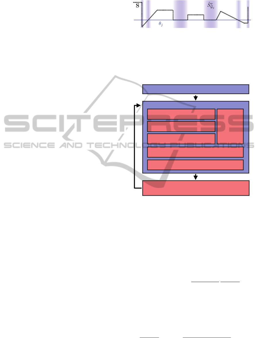
initialize a set of models by RANSAC
random jump
optimize labeling
accept randomly with distribution
according to energy gain
optimize model
j p
insert / delete model
swap model
split / merge model
compute
proposal
probabilities
based on
RANSAC
Figure 4: Overview of the presented algorithm.
the Markov chain to be Φ
o
, the probability of a move
Φ
o
AΦ
n
is:
P(Φ
o
AΦ
n
) = G(Φ
o
AΦ
n
)A(Φ
o
AΦ
n
) , (17)
where the move is proposed with the probability
G(Φ
o
AΦ
n
) and accepted with probability
A(Φ
o
AΦ
n
). Given a random proposal, the well-
known Metropolis choice defines the acceptance
probability to be (Suzuki, 1993):
A(Φ
o
AΦ
n
) = min
1,
G(Φ
n
AΦ
o
)
G(Φ
o
AΦ
n
)
p(Φ
n
|S)
p(Φ
o
|S)
.
(18)
The first term is the ratio of the proposal probabilities
G and describes the dynamic for selecting the move
Φ
o
AΦ
n
. If probabilities are expressed with respect
to the energy function U(Φ, S), the second fraction in
Equation 19 results in:
p(Φ
n
|S)
p(Φ
o
|S)
= exp (−
U(Φ
n
, S) −U(Φ
o
, S)
λT
) , (19)
where T is the temperature and λT simulates an an-
nealing behavior. T is decreased over time to allow
SemanticSegmentationandModelFittingforTriangulatedSurfacesusingRandomJumpsandGraphCuts
245

random jumps in the beginning of the optimization
procedure while the decisions become more deter-
ministic with increasing number of iterations (Lafarge
et al., 2013).
Figure 5: RANSAC-based computation of proposal prob-
abilities. Consider the parameter space for a geometric
model (θ
(1)
, θ
(2)
). The probability distribution p(M
j
|S)
for a geometric model given a triangulated surface segment
(blue line) is difficult to evaluate. However, RANSAC is
used to compute model candidates that can be seen as sam-
ples from the unknown distribution. Based on these sam-
ples, p(M
j
|S) is approximated by a kernel-based density
estimator.
Table 1: Overview of random moves and their correspond-
ing proposal probabilities. 1-2 are diffusion moves and 3-7
are implementing discrete jumps.
move proposals G(Φ
o
AΦ
n
)
1 opt. M
k
p(l
k
)
2 opt. X 1
3 split p(l
k
)p(M
i, j
|S
k
)
4 merge p(l
i
)p(l
j
|l
i
)p(M
k
|S
i, j
)
5 insert p(M
n
|S
u
)
6 delete p(l
k
)
7 swap p(l
k
)p(M
n
|S
k
)
5.1 Proposal Probabilities
One of the most crucial aspects in the design of
an MCMC process is the computation of the pro-
posal probabilities. In the original paper by Metropo-
lis et al. a uniform distribution is assumed. This
means that, given a current state Φ
o
, every state Φ
n
within a bounding box of Φ
i
is equally likely. How-
ever, this leads to a slow convergence since the ratio
p(Φ
n
)p(Φ
o
)
−1
is close to zero for most of the pro-
posed states (only a small subset yields high station-
ary probability). On the other hand, if randomized
choices are replaced by deterministic decisions, the
algorithm degenerates to a greedy method. A set of
seven moves are defined for the stated problem (1-2
diffusion, 3-7 jumps). A move is selected randomly
according to a uniform distribution. Each move re-
quires a sequence of randomized decisions. The pro-
posal probabilities for each move are given in Table
1.
5.1.1 Optimize Model (Diffusion)
A model M
k
is randomly chosen according to p(l
k
).
The computation of p(l
k
) is explained in Section
5.1.6. Given a fixed partition S
k
∈ S, the parameters
θ
k
are optimized based on the gradient
∂U
D
(Φ,S)
∂θ
k
. In
this work, a standard Levenberg-Marquardt algorithm
is used to optimize the model parameters.
5.1.2 Optimize Labeling (Diffusion)
The second diffusion move is used to minimize the
energy of the prior term in Equation 9. If the model
O is assumed to be fixed, the energy function can
be minimized by graph cuts. We perform one α-
expansion iteration to compute the labeling X (De-
long et al., 2010). The method allows to optimize spa-
tially regularized classification problems while mini-
mizing the number of used labels. A class l
k
yields
label costs as soon as at least one site in X is as-
signed with this label. This nicely allows to incorpo-
rate model complexity into the random-jumps frame-
work.
5.1.3 Split and Merge Model (Jump)
Given a randomly selected class l
k
, two new mod-
els M
i, j
are proposed according to p(M
i, j
|S
k
).
p(M
i, j
|S
k
) is computed based on a data-driven ap-
proach which is described in Section 5.2. The com-
plementary move is to merge two regions which are
randomly chosen according to p(l
i
)p(l
j
|l
i
). In order
to estimate p(l
j
|l
i
), we consider all segments which
are adjacent to S
i
. on S. Finally, RANSAC is used to
compute p(M
k
|S
i, j
).
5.1.4 Insert New and Delete Old Models (Jump)
All vertices which could not been assigned to exist-
ing models with a data cost below c
A
are assigned to
the default class A. The set of all vertices v ∈ S
A
is
used to propose new models according to p(M
n
|S
A
).
The delete move selects an existing model by p(l
k
)
for removal.
5.1.5 Swap Model (Jump)
The swap move allows to switch between different
types of models. This includes to select an existing
model p(l
k
) and propose a new model p(M
n
|S
k
) using
RANSAC. Note that the choice of the target model
M
n
is independent of the former model M
k
.
VISAPP2015-InternationalConferenceonComputerVisionTheoryandApplications
246
5.1.6 Selecting a Candidate
A component k which is considered in a move is se-
lected according to p(l
k
). Instead of assuming a uni-
form distribution, p(l
k
) could also be estimated with
respect to the size of the underlying segment |S
k
|. A
larger segment is more likely to be described by two
instead of only one model. Two smaller segments,
however, might yield a lower energy if they are repre-
sented by one common model. However, this is only
a heurisitic which does not turn out to be significantly
better than a uniform distribution in our experiments.
5.2 Data-driven Proposals
Even if a very limited set of moves is considered,
the likelihood of decreasing Equation 6 significantly
depends on p(M |S). The Data-driven method pro-
posed by Tu and Zhu uses bottom-up algorithms to
estimate p(M |S) such that this is close to the actual
probability density (Tu and Zhu, 2002). We want to
adapt that method for our purpose. Methods such as
RANSAC might not always compute a certain opti-
mum but ”proposals” of such methods are likely to
decrease p(Φ|S). In this work, the algorithm of Schn-
abel et al. is modified for the domain of triangulated
surfaces. The algorithm is referred to as Γ. Suppose
that S is a subset of the triangulated surface S ∈ S
and θ
Γ
= {e
ε
, n
ε
} is a set of parameters which signif-
icantly influence the result. The e
ε
-environment and
the maximally allowed normal deviation n
ε
are the in-
lier thresholds for the RANSAC procedure. The re-
maining parameters are set to the proposed standard
values. Please refer to the corresponding paper for
further details (Schnabel et al., 2007). The optimal set
for θ
Γ
is not known and a random sample θ
Γ
∼ p(θ
Γ
)
is drawn to generate a set of shape candidates:
{M
k
∈ G} = Γ(S, θ
Γ
) . (20)
Each candidate is associated with a weight ω
k
which
is a normalized sum of over all vertices belonging to
the considered segment S:
ω
k
=
1
|S|
∑
v∈S
p(v|M
k
) , (21)
where p(v|M
k
) is the likelihood of v belonging to M
k
.
p(v|M
k
) can also be interpreted as a vote of v for M
k
.
In order to fulfill the requirements of a MCMC pro-
cess, all possible configurations of M
k
should have
p(M
k
|S) > 0:
p(M
k
|S) =
1
∑
|G|
i=0
ω
i
∑
|G|
ω
i
K(θ
k
− θ
i
) , (22)
where K() is a kernel function such as Parzen window.
p(M ) > 0 is required for the ergodicity of the Markov
chain. The computation of the proposal probabilities
is visualized in Figure 5.
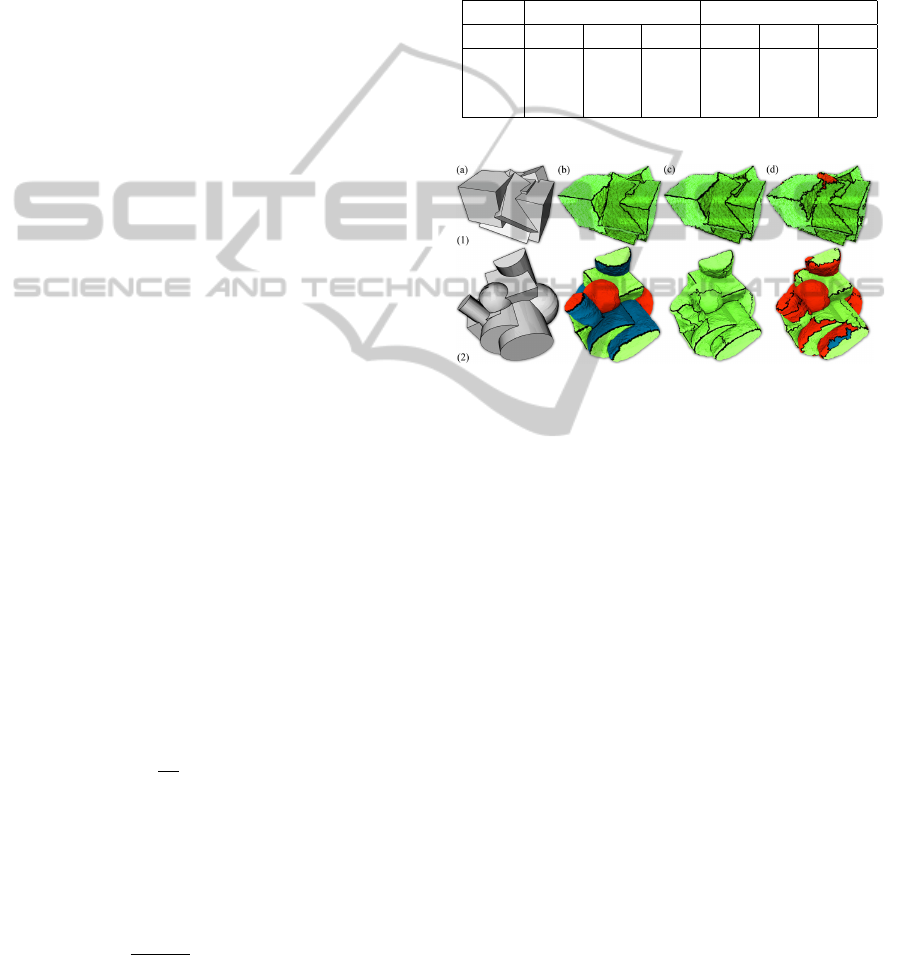
Table 2: Segmentation score for the three considered algo-
rithms, random jumps (b), variational shape approximation
(c), and hierachical clustering (d). The number in each cell
represents the normalized score of a segmentation. A ver-
tex contributes a positive value to the overall score if cor-
rectly assigned to the most overlapping segment. The over-
all score is given as percent per total number of vertices.
Mdl. Planar Mixed
Alg. N1 N2 N3 N1 N2 N3
(b) 85.4 71.8 70.4 87.1 82.0 80.7
(c) 80.7 63.1 62.9 45.0 40.2 38.2
(d) 81.8 61.2 57.5 73.0 57.9 54.9
Figure 7: Visual comparison of the segmentation for two
synthetic data sets. Row (1) shows the result for the planar
model (N1) and row (2) for the mixed model (N2). Each
row starts with the original, synthetic CAD model (a), fol-
lowed by the resulting segmentation of the three considered
algorithms, random jumps (b), variational shape approxi-
mation (c), and hierarchical clustering (d). In the table be-
low, the number in each cell represents the normalized score
of a segmentation. A vertex contributes a positive value to
the overall score if correctly assigned to the most overlap-
ping segment. The overall score is given as percent per total
number of vertices.
6 EVALUATION
The presented algorithm is qualitatively and quanti-
tatively compared to two related approaches. The
greedy algorithm presented by Attene et al. performs
segmentation by fitting spheres, cylinders and planes
in a hierarchical clustering scheme (Attene et al.,
2006). Driven by Lloyd’s algorithm, the variational
framework introduced by Cohen-Steiner et al. decom-
poses a mesh in approximately planar regions based
on the normal vectors (Cohen-Steiner et al., 2004).
6.1 Qualitative Comparison
Both competitive methods require the number of clus-
ters to be specified manually. In this experiment, it is
SemanticSegmentationandModelFittingforTriangulatedSurfacesusingRandomJumpsandGraphCuts
247
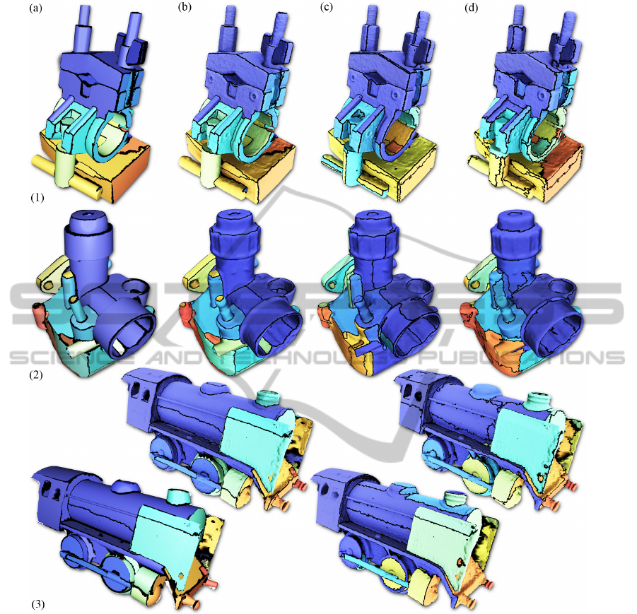
Figure 6: Result of the qualitative comparison for three different models, Clamp (1), Carburetor (2), and Train (3). The result
of our method is shown in (a) and (b). (a) visualizes the synthesized model while the segmentation is shown in (b). The results
for the segmentation algorithm based on hierarchical clustering can be found in (c), while the outcome of the variational shape
approximation is shown in (d).
set according to the number of components extracted
by our algorithm. For the entire qualitative evalua-
tion, α = 1000, β = 20 are used as prior parameters.
The result of the qualitative evaluation can be seen in
Figure 6. We apply the considered methods to three
different models that have been acquired by the 3D
reconstruction tool chain proposed by Jancosek et al.
: Clamp (1), Carburetor (2), and Train (3) (Jancosek
and Pajdla, 2011). The result of the presented method
is shown in the first two rows. The synthesized object
O is visualized in (a) and the semantic segmentation
X is presented in (b). It can clearly be seen, that the
O captures the most important geometric features of
the model that allow to decompose S into smooth seg-
ments. The boundary curves (black) are free of per-
turbations and run along the principle curvature direc-
tions. Due to the prior term, O balances fitting qual-
ity and model complexity. The variational approach
decomposes the surface according to the normal vec-
tors which leads to approximately planar segments
(c). If the model consists of planar segments which
are separated by sharp feature lines, the variational
approach delivers satisfying results, as it is shown in
(1,c). However, the partition step is driven by region
VISAPP2015-InternationalConferenceonComputerVisionTheoryandApplications
248
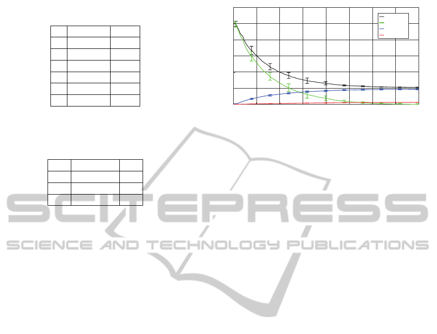
Table 3: Overview of the label costs for all considered
model types.
type |M
k
|
1 plane 2
2 cylinder 6
3 sphere 8
4 torus 10
5 cone 10
7 default 1
Table 4: The intensity of the noise is given by the ratio of the
maximal deviation and the global scale of the data. In this
work, we apply fractal Brownian motion (fBm) and ridged
multifractal noise (rmf).
noise r
σ
N1 fBm .02
N2 rmf .04
N3 fBm+rmf .06
growing which leads to scattered segment boundaries
on less curved regions of the surface (bottom region in
(1,c)) . The result of the Lloyd algorithm also depends
on the initialization of the clusters. Another problem
are small, degenerated segments (black dots in (2,c)
and (3,c)). This problem remains even when seeds
are ”teleported” as suggested in the paper of Cohen-
Steiner et al. The hierarchical clustering algorithm
is very sensitive to noise and produces very scattered
boundary curves, especially on approximately flat re-
gions of the surface. Due to its greedy nature, it fails
to reasonably decompose the surface into spherical
and cylindrical regions as it can be seen in (2,d).
The convergence behavior of the MCMC process
for the Carburetor model is plotted in Figure 8 for
ten optimizations. The graph shows the mean and
the variance for the total energy (Equation 6) as well
as for the three components, data costs (Equation
10), smoothness (Equation 8), and model complex-
ity (Equation 7). For each run, the algorithm is ini-
tialized with four randomly detected primitives. The
energy clearly converges to a minimum.
6.2 Quantitative Comparison
In a second experiment, we use two CAD models
as ground truth and simulate the measurement pro-
cess by surface reconstruction and random deforma-
tion. Using Boolean operations, the planar model is a
union of boxes while the mixed model is composed of
boxes, cylinders, and spheres. This yields a decompo-
sition into faces that can be described by bounded ge-
ometric primitives. The CAD models are sampled at
a very high resolution to obtain a set of reference ver-
tices (> 1m). A standard surface reconstruction algo-
0 50 100 150 200 250 300 350 400
0
0.5
1
1.5
2
2.5
3
x 10
7
mean energy vs iterations clamp model
iteration
mean energy
total energy
data
label
smooth
Figure 8: Convergence behavior for the clamp model. The
plot shows mean and covariance of the energies for ten op-
timization processes. The total energy (black) is composed
of data (green), label (blue), and smoothing costs (red). The
algorithm was initialized with random settings for each run.
rithm is then applied to compute a test mesh which is
used as input data for the algorithms. We apply fractal
Brownian motion (fBm) and ridged multifractal noise
(rmf) to randomly deform the test mesh at different
intensity levels (Ebert, 2003). Please refer to Table 4.
The intensity is given as the ratio r
σ
of the maximal
deviation and the global scale of the test mesh. After
applying the algorithm, a score is computed by com-
paring the estimated labels with the ground truth for
each vertex. Since we do not have explicit classes, we
compute a unique mapping between estimated labels
and ground truth data such that the overlap is maxi-
mized. A vertex contributes one to the overall score if
correctly classified, otherwise zero. The normalized
score is given in Table 2. 100 means all vertices in
the test mesh are correctly classified, zero means no
vertex is classified correctly. The score is the aver-
age of ten runs per algorithm. The number of clusters
is manually specified to be the true number of clus-
ters for both competing algorithms. The results are
also presented for visual inspection in Figure 7. In
(1), the segmentation is applied to the planar model
(N1). The result for the mixed model that is deformed
by rmf noise (N2) is shown in (2). The presented
algorithm outperforms the other methods in all cat-
egories. However, both competitive algorithms also
show a feasible performance at the lowest noise level.
The performance of the hierarchical clustering algo-
rithm drastically decreases with higher noise levels.
The score for the variational algorithm mainly suffers
from the sensitivity to bad cluster initializations.
7 CONCLUSION
A new and robust approach for the simultaneous clas-
sification and model fitting for triangulated surfaces is
presented. The problem is formulated as a minimiza-
SemanticSegmentationandModelFittingforTriangulatedSurfacesusingRandomJumpsandGraphCuts
249

tion of a global energy function. A MCMC frame-
work allows to robustly compute a solution that ex-
plains the measured data. RANSAC turns out to be
very efficient for computing new proposals that are
likely to minimize the energy function. In future re-
search, the algorithm will be extended by more ad-
vanced models, such as b-spline patches or quadrics
surfaces.
REFERENCES
Attene, M., Falcidieno, B., and Spagnuolo, M. (2006). Hi-
erarchical mesh segmentation based on fitting primi-
tives. The Visual Computer, 22:181–193.
Benhabiles, H., Lavou
´
e, G., Vandeborre, J.-P., and Daoudi,
M. (2011). Learning boundary edges for 3d-mesh seg-
mentation. In Computer Graphics Forum, volume 30,
pages 2170–2182. Wiley Online Library.
Cohen-Steiner, D., Alliez, P., and Desbrun, M. (2004). Vari-
ational shape approximation. In ACM Transactions on
Graphics, volume 23, pages 905–914. ACM.
Delong, A., Osokin, A., Isack, H., and Boykov, Y. (2010).
Fast approximate energy minimization with label
costs. In 2010 IEEE Conference on Computer Vision
and Pattern Recognition, pages 2173–2180.
Ebert, D. S. (2003). Texturing & modeling: a procedural
approach. Morgan Kaufmann.
Han, F., Tu, Z., and Zhu, S.-C. (2004). Range image
segmentation by an effective jump-diffusion method.
IEEE Transactions on Pattern Analysis and Machine
Intelligence, 26(9):1138–1153.
Isack, H. and Boykov, Y. (2012). Energy-based geomet-
ric multi-model fitting. International Jorunal of Com-
puter Vision, 97(2):123–147.
Jancosek, M. and Pajdla, T. (2011). Multi-view recon-
struction preserving weakly-supported surfaces. In
2011 IEEE Conference on Computer Vision and Pat-
tern Recognition, pages 3121–3128. IEEE.
Kalogerakis, E., Hertzmann, A., and Singh, K. (2010).
Learning 3d mesh segmentation and labeling. In ACM
SIGGRAPH 2010 Papers, SIGGRAPH ’10, pages
102:1–102:12, New York, NY, USA. ACM.
Lafarge, F., Keriven, R., Br
´
edif, M., and Vu, H.-H. (2013).
A hybrid multiview stereo algorithm for modeling ur-
ban scenes. IEEE Transactions on Pattern Analysis
and Machine Intelligence, 35(1):5–17.
Lai, Y.-K., Hu, S.-M., Martin, R. R., and Rosin, P. L. (2008).
Fast mesh segmentation using random walks. In Pro-
ceedings of the 2008 ACM symposium on Solid and
physical modeling, pages 183–191. ACM.
Lavou
´
e, G. and Wolf, C. (2008). Markov random fields
for improving 3d mesh analysis and segmentation. In
3DOR, pages 25–32.
Li, Y., Wu, X., Chrysathou, Y., Sharf, A., Cohen-Or, D.,
and Mitra, N. J. (2011). Globfit: Consistently fitting
primitives by discovering global relations. In ACM
Transactions on Graphics (TOG), volume 30, page 52.
ACM.
Longjiang, E., Waseem, S., and Willis, A. (2013). Using
a map-mrf model to improve 3d mesh segmentation
algorithms. In Southeastcon, 2013 Proceedings of
IEEE, pages 1–7. IEEE.
Lv, J., Chen, X., Huang, J., and Bao, H. (2012). Semi-
supervised mesh segmentation and labeling. In Com-
puter Graphics Forum, volume 31, pages 2241–2248.
Wiley Online Library.
Mangan, A. P. and Whitaker, R. T. (1999). Partitioning 3d
surface meshes using watershed segmentation. IEEE
Transactions on Visualization and Computer Graph-
ics, 5(4):308–321.
Papazov, C. and Burschka, D. (2011). An efficient
ransac for 3d object recognition in noisy and occluded
scenes. In Kimmel, R., Klette, R., and Sugimoto, A.,
editors, Computer Vision ACCV 2010, volume 6492
of Lecture Notes in Computer Science, pages 135–
148. Springer Berlin Heidelberg.
Schnabel, R., Wahl, R., and Klein, R. (2007). Efficient
ransac for point-cloud shape detection. Computer
Graphics Forum, 26(2):214–226.
Suzuki, M. (1993). Quantum Monte Carlo methods in con-
densed matter physics. World scientific.
Tu, Z. and Zhu, S.-C. (2002). Image segmentation by data-
driven markov chain monte carlo. IEEE Transac-
tions on Pattern Analysis and Machine Intelligence,
24(5):657–673.
V
´
arady, T., Facello, M. A., and Ter
´
ek, Z. (2007). Automatic
extraction of surface structures in digital shape recon-
struction. Computer Aided Design, 39(5):379–388.
Woodford, O. J., Pham, M.-T., Maki, A., Gherardi, R., Per-
bet, F., and Stenger, B. (2012). Contraction moves for
geometric model fitting. In Proceedings of the 12th
European Conference on Computer Vision - Volume
Part VII, ECCV’12, pages 181–194, Berlin, Heidel-
berg. Springer-Verlag.
Wu Leif Kobbelt, J. (2005). Structure recovery via hy-
brid variational surface approximation. In Computer
Graphics Forum, volume 24, pages 277–284. Wiley
Online Library.
Yan, D.-M., Wang, W., Liu, Y., and Yang, Z. (2012). Vari-
ational mesh segmentation via quadric surface fitting.
Computer-Aided Design, 44(11):1072–1082.
VISAPP2015-InternationalConferenceonComputerVisionTheoryandApplications
250
