
CEFM
A Heuristic Mesh Segmentation Method based on Convexity Estimation and Fast
Marching
Jun Zhang
1,2
, Zhouhui Lian
1
, Zhenbao Liu
2
and Jianguo Xiao
1
1
Institute of Computer Science and Technology, Peking University, Beijing, P.R.China
2
School of Aeronautics, Northwestern Polytechnical University, Xi’an, P.R.China
Keywords:
Mesh Segmentation, Shape Descriptor, Convexity, Fast Marching, Local Depth.
Abstract:
Mesh segmentation is a fundamental way of shape analysis and understanding for 3D mesh models. In this pa-
per, we propose an effective heuristic mesh segmentation algorithm, which is based on concave areas detection
and heuristic 2-category classification via fast marching. The algorithm has several merits. First, the boundary
between each pair of segments is close to the natural seams of 3D objects. Second, it is robust against pose
variations and isometric transformations. Finally, our algorithm decomposes non-rigid 3D models into a set
of rigid components in a short period of time and the procedure is fully automatic. Extensive experiments in
this paper demonstrate that the proposed method outperforms the state of the art in mesh segmentation.
1 INTRODUCTION
3D mesh models are now widely available and used
in various applications due to the rapid development
of 3D acquisition techniques. As a result, the demand
for mesh analysis and understanding is ever increas-
ing. Segmenting 3D models into parts with semantic
information is a fundamental problem in geometric
processing. Many relevant tasks such as shape re-
trieval, skeleton extraction, mesh editing and so on,
require mesh segmentation as a preprocessing step.
However, until now, how to automatically and prop-
erly segment 3D models into parts which are consis-
tent with human perception is still a challenging prob-
lem.
In (Shapira et al., 2008), the authors proposed a
novel local shape descriptor named shape-diameter
function (SDF) and applied it to mesh segmentation.
The SDF descriptor describes volumetric information
of mesh models by measuring the diameter of lo-
cal parts, which helps to guide volumetric part ex-
traction and shape segmentation. The major limita-
tion of SDF-guided segmentation is that it is not able
to decompose non-rigid parts with similar volumet-
ric information (e.g., in Fig.3(d), two thighs of a hu-
man model are not separated), most of which is un-
desirable for human perception and real applications.
Lai et al.(Lai et al., 2008) extended the original ran-
dom walks segmentation method from 2D images to
3D meshes. The main idea of this work is to automat-
ically select a couple of seeds (representing the labels
of different parts) from a mesh model to achieve over-
segmentation, and then merge the parts based on the
similarity of neighboring parts. The method is fast
and easy to implement, but it tends to over segment
most of the mesh models, which goes against human
perception.
Inspired by the aforementioned methods, we de-
sign an effective automatic segmentation algorithm.
Specifically, we improve the SDF-guided segmenta-
tion method and use it as an initial segmentation pro-
cess, and then propose a heuristic algorithm to im-
plement further segmentation of subparts. The lat-
ter is based on the detection of concave areas and 2-
category classification. The basic idea of our heuristic
algorithm is to firstly set a criterion to estimate each
segmented part obtained after the initial segmentation
process and decide whether it should be further seg-
mented or not. If the criterion is satisfied, the part will
then be further segmented by a fast-marching-based
method (see Section 3.2.3). The algorithm repeats
this procedure until there is no change in any seg-
mented part. We have tested our method elaborately
with the Princeton Segmentation Benchmark (Chen
et al., 2009) and the experimental results indicate that
our method outperforms the state-of-the-art methods.
The remainder of this paper is organized as follows.
Section 2 briefly reviews related work. An effective
114
Zhang J., Lian Z., Liu Z. and Xiao J..
CEFM - A Heuristic Mesh Segmentation Method based on Convexity Estimation and Fast Marching.
DOI: 10.5220/0005265801140121
In Proceedings of the 10th International Conference on Computer Graphics Theory and Applications (GRAPP-2015), pages 114-121
ISBN: 978-989-758-087-1
Copyright
c
2015 SCITEPRESS (Science and Technology Publications, Lda.)
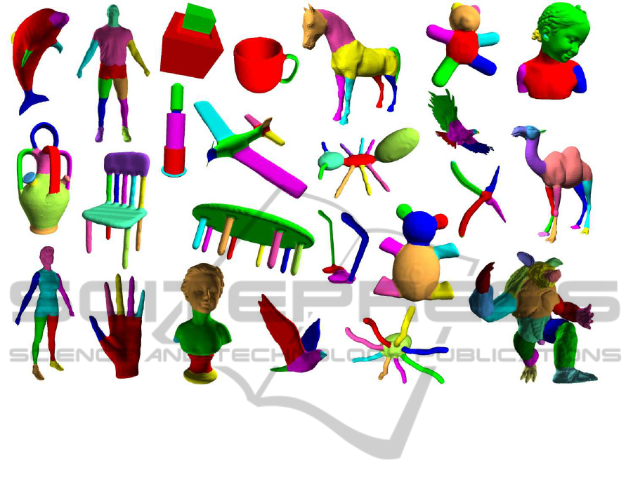
Figure 1: Segmentation results of representative models in the Princeton Segmentation Benchmark (Chen et al., 2009) using
our proposed method. It can be clearly seen that our segmentation boundaries naturally follow the seams of shapes.
mesh segmentation algorithm based on concave ar-
eas detection and heuristic 2-category classification is
presented in Section 3. Experimental results and dis-
cussions are given in Section 4, following with con-
clusions in Section 5.
2 RELATED WORK
Generally, existing mesh segmentation methods can
be classified into two categories based on the types
of models they aim to segment. Algorithms of the
first category are designed for applications such as re-
verse engineering of CAD models. These methods
segment models into patches, and each patch is con-
sidered as the best fit to one of the given mathematical
surfaces, such as planes, cylinders and spheres, etc.
The second category consists of algorithms that con-
centrate on segmenting natural shapes into semantic
components which correspond well with human intu-
ition. Our algorithm mainly aims at solving the latter
problems.
Numerous approaches for 3D shapes segmenta-
tion have been explored in the last few years. For
instance, Shlafman et al. (Shlafman et al., 2002)
used k-means clustering to segment the models into
meaningful parts. Katz et al. (Katz et al., 2003)
improved the above-mentioned approach by using
fuzzy clustering and graph cut methods to achieve
smoother boundaries between clusters. These meth-
ods are mainly based on iterative clustering, which
can be easily achieved. But the necessity to com-
pute pairwise distances makes them computationally
expensive to handle high-resolution models directly.
To solve this problem, Zhang and Liu (Zhang and
Liu, 2005), (Liu and Zhang, 2007) employed spectral
clustering methods to analyze meshes in 2D space.
While Lai et al. (Lai et al., 2008) extended random
walks method originally used for image segmentation
to the mesh segmentation problem. A common fea-
ture of the methods mentioned above is that they all
include concavity information in their underlying al-
gorithm, which ensures that the boundaries between
segmented parts adhere to concave areas. However,
all these methods use a single set of seeds or clus-
ter centers to guide the segmentation procedure. As
a result, they rely heavily on the number of seeds or
clusters.
There also exist some other more complex meth-
ods for mesh segmentation. For example, Katz et
al. (Katz et al., 2005) proposed a method based on
core extraction using centricity information to deter-
mine the prominent parts of the models. The ran-
domized cuts method was proposed in (Golovinskiy
and Funkhouser, 2008) to generate a random set of
CEFM-AHeuristicMeshSegmentationMethodbasedonConvexityEstimationandFastMarching
115

mesh segmentationsand then measure how often each
edge of the mesh lies on a segmentation boundary in
the randomized set to accomplish final segmentation.
Kalogerakis et al. (Kalogerakis et al., 2010) trained
a conditional random field probabilistic model for si-
multaneous segmentation and labeling of parts in 3D
meshes. They fused hundreds of informative features
such as curvature, shape context, etc, in the train-
ing procedure to achieve good segmentation perfor-
mance. Nevertheless, most of these alternative meth-
ods involve complicated procedures, which result in
high computation cost.
Our method employs a modified SDF-guided seg-
mentation method as an initial segmentation process,
which is fast and effective for coarse partition of
mesh models. After that, a heuristic algorithm based
on convexity estimation and fast marching methods
(Sethian, 1999) is utilized to implement further sub-
parts segmentation. Compared to methods mentioned
above, the method proposed in this paper is robustand
effective with less parameters and low computation
cost.
3 METHOD DESCRIPTION
3.1 Initial Segmentation
As mentioned in Section 1, the first step of our method
is to implement an initial segmentation procedure.
The aim of this procedure is to decompose any mesh
model into a principal part and other branch parts in
a coarse way. One reason why we do this initial seg-
mentation is to avoid over-segmentation and bad seg-
ment boundaries, as the heuristic strategy is difficult
to control when the mesh model is complex in topo-
logical structure. Another reason is that, with the ini-
tial segmentation process, the time costs of the whole
algorithm can be markedly reduced. In other words,
the initial segmentation step takes charge of the gen-
eral decomposition while the heuristic segmentation
step executes the detailed work.
When segmenting 3D meshes, we observe that the
subparts of a given model to be separated contain cer-
tain volumetric information, which is distinguishable
among different subparts. Therefore, a proper solu-
tion is needed to capture these volumetric information
for segmentation. We employ an efficient segmenta-
tion procedure by utilizing shape diameter function
(SDF) (Shapira et al., 2008) descriptor (see Fig.2).
The SDF descriptor connects volumetric information
of a mesh model onto its boundary mesh by measur-
ing the local diameter of the model at faces on its
boundary. Hence, it is suitable to guide volumetric
part extraction and shape segmentation.
Figure 2: Some typical models from the Princeton Segmen-
tation Benchmark model set. The color mapping on the
models is the normalized SDF values. As we can see that
these values are able to indicate similarity between analog
parts.
Specifically, our method first builds a Gaus-
sian Mixture Model (GMM) with the Expectation-
Maximization (EM) (Bilmes, 1997) algorithm to fit
k Gaussian functions to the histogram of SDF values
of faces on the mesh. By using GMM, we can com-
pute a vector v
f
∈ R
k
for each face f, where v
i
f
is the
probability of f belonging to the ith Gaussian func-
tion. Here, k is experimentally chosen as 3 for most
models. For some models with simple topological
structure, the value is set to k = 2. If simply choosing
the most probable index of Gaussian function to label
each f, we can obtain an initial result as demonstrated
in Fig.3(b). This is undesirable because it doesn’t in-
clude contextual information and thus results in large
numbers of holes and jags.
To improve the initial segmentation results ob-
tained above, we take contextual information of the
mesh into account and make sure that the boundaries
between segmented parts are smooth and approach lo-
cal mesh features such as concave areas or creases.
We employ an alpha expansion graph-cut algorithm
(Boykov et al., 2001) to fulfil the goal. The graph cut
procedure assigns a single segment label to each face,
considering both the probability vector from the EM
step and the contextual information. Specifically, The
graph cut procedure minimizes the following energy
function:
E( ˆx) =
∑
f∈F
e
1
( f, ˆx( f )) + λ
∑
( f,g)∈E
e
2
( ˆx, f, g)+ (1)
µ
∑
( f,g)∈E
e
3
( ˆx, f,g),
e
1
( f, ˆx( f)) = −log(P( f| ˆx( f)) + ε), (2)
GRAPP2015-InternationalConferenceonComputerGraphicsTheoryandApplications
116
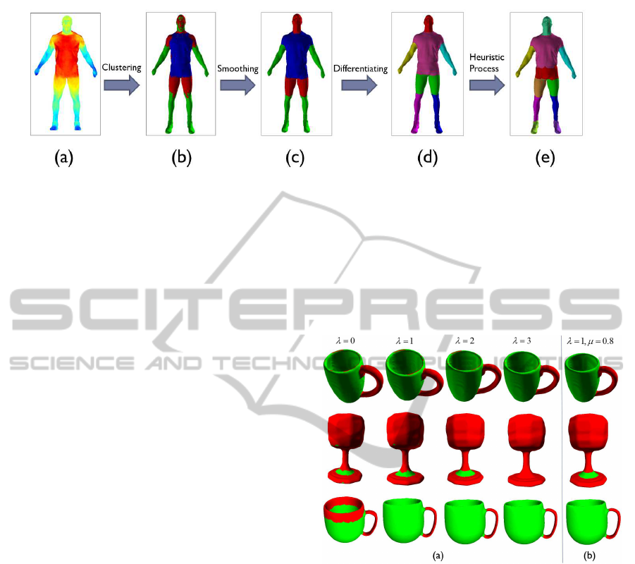
Figure 3: Process of our segmentation method. (a) Distribution of the SDF values. (b)Result of clustering only. (c) Modified
segmentation with contextual information. (d) Differentiating the similar parts. (e) The final segmentation result.
e
2
( ˆx, f,g) =
l
( f,g)
(1− log(θ
( f,g)
/π)) ˆx( f) 6= ˆx(g),
0 ˆx( f) = ˆx(g),
(3)
e
3
( ˆx, f,g) =
l
( f,g)
(1− log(d
( f,g)
+ ε)) ˆx( f) 6= ˆx(g),
0 ˆx( f) = ˆx(g),
(4)
where
• ˆx denotes the face label.
• P( f| ˆx( f)) refers to the probability of assigning
face f to label ˆx( f). These values are derived
from the normalized summation values.
• θ
( f ,g)
represents the dihedral angle between any
connected pair of faces f and g.
• d
( f ,g)
represents the difference between SDF val-
ues of any connected pair of faces f and g.
• l
( f ,g)
is the length of the edge shared by f and g.
• F and E are the face set and edge set respectively.
• λ, µ and ε are constants. Experimentally, we set λ
to 1, µ to 0.8 and ε to 10
−3
.
We consider e
1
as a data term, e
2
and e
3
as
smoothness terms. Note that the main difference be-
tween our method and the original one proposed in
(Shapira et al., 2010) is the introduction of e
3
, which
is of great significance in improving the segmenta-
tion results. e
2
helps to contract the boundaries be-
tween parts to the concave areas. However, if we put
more emphasis on e
2
(by increasing the value of λ),
most of the correctly-segmented parts will merge to-
gether. On the other hand, the segmentation result
won’t be smooth and will attach with many undesired
little patches if we assign λ with a small value (see
Fig.4(a)). We introduce e
3
to play a role as a trade-
off to fix this problem. The e
3
term measures how
similar each pair of adjacent faces is based on the dis-
similarity between their features. Under the impact
of e
3
, labels of any adjacent faces will stay the same
if the feature distance between them is small enough.
Otherwise, they will be different. The effectiveness of
e
3
is demonstrated in Fig.4(b). As shown in Fig.9, our
further experiments verify that the e
3
term contributes
greatly to the final segmentation results.
Figure 4: Our initial segmentation results of some cup mod-
els over a range of parameters. (a) The parameter λ of
smooth term e
2
ranging from 0 to 3. We can see that the val-
ues of λ suitable for various models arenot always the same.
(b) Combined action of smooth term e
2
and e
3
. With the
help of e
3
, the initial segmentation results become smoother
and more robust.
After above-mentioned procedures, we observe
that similar parts are still assigned with the same la-
bels, see Fig.3(c). We obtain the actual parts via
propagating from a seed face to differentiate the parts
which are not connected but with the same label. Up
to now, the final results of initial segmentation process
have been acquired (see Fig.3(d)).
3.2 Heuristic Segmentation
As previously mentioned, the goal of the initial seg-
mentation process is to coarsely decompose any mesh
model into a principal part and other branch parts.
CEFM-AHeuristicMeshSegmentationMethodbasedonConvexityEstimationandFastMarching
117
For example, a human model will be partitioned into
torso, head, arms and legs after the initial processing.
However, it is far from being enough to achieve a bet-
ter and natural segmentation result and reach the goal
to decompose a non-rigid 3D model into a set of rigid
components. Thereby, we design a heuristic segmen-
tation procedure to execute further decomposition for
those initially segmented parts.
3.2.1 Criterion for Part-segment
Each part in a certain model obtained after the initial
segmentation process should be estimated whether to
be segmented again or not. Our strategy is to calculate
the convexity value of each part and set a threshold.
If the convexity value is under the threshold, then this
part is suggested to be segmented again. Otherwise
it remains the same. Numerous experimental results
demonstrate that the most appropriate threshold value
can be selected as 0.85. The convexity value C of a
part P is defined as follows,
C(P) =
Volume(P)
Volume(CH(P))
, (5)
where CH(P) is the convex hull of part P. As il-
lustrated in Fig.5 which shows the volume of each
part and the corresponding convex hull of a human
model, we can easily decide which parts should be
segmented again (i.e., crus, thigh and torso maybe)
or not (i.e., head and hands). Therefore, the criterion
defined above is able to make sure that all non-rigid
parts can be segmented again.
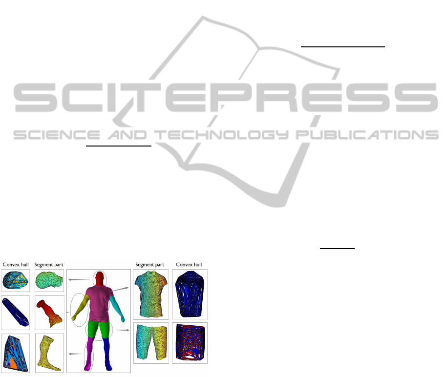
Figure 5: Overview of segment parts of a human model.
In the center is an initial segmentation result of the human
model, and on both sides are segmented parts and their cor-
responding convex hulls.
3.2.2 Local Depth
The local depth (Lin et al., 2010) feature measures
how deep a position is located with respect to its
neighbors. The basic idea of local depth comes from
the observation of Fig.6(b) . As we can see, there is
an obvious height difference between D and E, but
the height difference between D and A is more suit-
able to measure the location of point D according to
human perception. One effective way of presenting
this feature is to calculate its local depth.
There are four steps to compute the local depth
of a given vertex v on a mesh M. For each ver-
tex on a mesh, we first determine its height direction
on its normal direction. The normal of a vertex is a
weighted sum of normals of its adjacent faces. Sup-
pose F
v
= { f | f is the face adjacent to v}, then the
normal of v can be estimated as
~n
v
=
∑
f
i
∈F
v
~n(f
i
) · Area( f
i
)
∑
f
i
∈F
v
Area( f
i
)
, (6)
Then we define the local neighbour. In Fig.6(b), if
we only consider one ring neighborhood, the depth of
point D is the difference between the heights of E and
D. But if we consider a wider range of neighborhood,
such as three rings, then the depth of point D becomes
the difference between A and D, which is more rea-
sonable. we set the ring number value to 3 in all the
experiments and obtain satisfactory results. Thirdly,
for each vertex v, we compute the height differences
between v and its neighbors to form the set D
v
=
{ d
uv
| d
uv
is the height difference between v and u }.
The height difference d
uv
is computed using Eq.7.
Finally, We select the largest value from D
v
as the
local depth of v.
d
uv
= cosα · |~uv| =
~n
u
· ~uv
|~n
u
| · |~uv|
· |~uv| =~n
u
· ~uv, (7)
From the definition of local depth, we can observe
that, firstly, a positive local depth indicates that the
vertex is at the concave position, and a negative one
indicates convex position. Secondly, the larger the
positive local depth of a vertex is, the more possible it
is for the vertex to be a boundary point, as the surface
is more bent, see Fig.6(a). The local depth feature
has been proved to consider a wider range of geom-
etry information than the curvature feature does via
large amounts of experiments conducted in (Lin et al.,
2010).
3.2.3 Fast-marching Based Segmentation
The ultimate goal of our method is to decompose any
non-rigid 3D model into a set of rigid components,
meanwhile ensuring that the boundary between each
pair of segmented parts should be very close to the
natural seams of the model. To achieve this goal, we
implement a further segmentation processing if a cer-
tain part, which comes from the initial segmentation
GRAPP2015-InternationalConferenceonComputerGraphicsTheoryandApplications
118
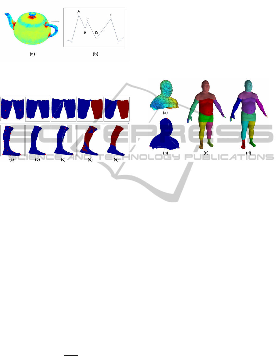
Figure 6: (a) The distribution of local depth values of a
teapot model. Vertices in the concave place of the mesh
have large local depth values, which are in red color. (b)
Schematic diagram of local depth.
Figure 7: Demonstration of our heuristic segmentation. (a)
Points sampling. (b) Seed points selection. (c) Pathways of
an arbitrary point towards both the seeds. (d) Labeling ac-
cording to the pathway local depth summation. (e) Smooth-
ing the labeling result.
process, satisfies the convexity estimation criterion.
There are mainly five steps in this procedure.
Uniform sampling. In this step, we need to com-
pute the geodesic distance between certain pairs of
vertices. As most of the mesh models we deal with
contain tens of thousands of vertices and faces, it’s
rather time-consuming and impractical to compute
the geodesic distance between any pair of vertices in a
model. As a result, we perform a uniform sampling to
obtain a certain number of vertices which are evenly
distributed in the segment part, as demonstrated in
Fig.7(a). we set the number of sample points to 20
in this paper.
Selecting seeds. Now we calculate both the
geodesic distance (based on fast marching methods
(Sethian, 1999)) and the Euclidean distance between
each pair of vertices in the sample point set. And then,
for each two sampled vertices, we calculate the ratio
between the geodesic distance and the Euclidean dis-
tance as follows,
r
uv
=
GD
uv
ED
uv
, (8)
where r
uv
is the distance ratio of vertices pair u and
v, GD denotes the geodesic distance and ED the Eu-
clidean distance. Then we sort the geodesic dis-
tance values calculated above in descending order,
and from the first ten pairs we choose a pair of ver-
tices as seeds whose distance ratio is the largest (see
Fig.7(b)). In most situations, the geodesic pathway
of this pair is able to cross the most bent area in the
segment part. We don’t simply choose the pair of ver-
tices with largest geodesic distance, because in certain
cases (e.g., Fig.8(c)) such processing results in incor-
rect segmentations while our results (e.g., Fig.8(d))
are satisfactory.
Figure 8: A special situation of a man model segmentation
procedure during seeds selection. (a) The upper body part
which is difficult to pick up the seeds. (b) Demonstration
of proper seeds selection. The pairs in both arms share the
largest geodesic distance, but the other pairs with larger dis-
tance ratio are supposed to be the seeds. (c) Segmentation
result without taking distance ratio into consideration. (d)
Segmentation result that is in consideration of distance ra-
tio.
Computing the Local Depth Summation. We com-
pute the geodesic pathway of every vertex to the seeds
using fast marching methods (Sethian, 1999). Then
for each vertex (except for seeds), we add up the lo-
cal depth values in each pathway to the seeds (see
Fig.7(c)).
Labeling the Part. We assign the two seeds with
different labels (e.g., 0 and 1). For each vertex, we
compare the summation values of each pathway. If
the pathway of a certain vertex to one of the seeds has
a smaller summation value, the label of this vertex
should be consistent with that of the seed, as shown
in Fig.7(d).
Smoothing the Result. As we can see from
Fig.7(d), in most cases, the labeling results do not
satisfy our requirements that the boundaries between
parts are smooth and adhere to concave areas or
creases. To address the problem, we employ the alpha
expansion graph-cut algorithm (Boykov et al., 2001)
again to smooth the labels. Different from the ini-
tial segmentation process, here we just use e
1
and e
3
to construct the smooth term in the energy function.
Fig.7(e) shows the final segmentation result after this
step.
CEFM-AHeuristicMeshSegmentationMethodbasedonConvexityEstimationandFastMarching
119
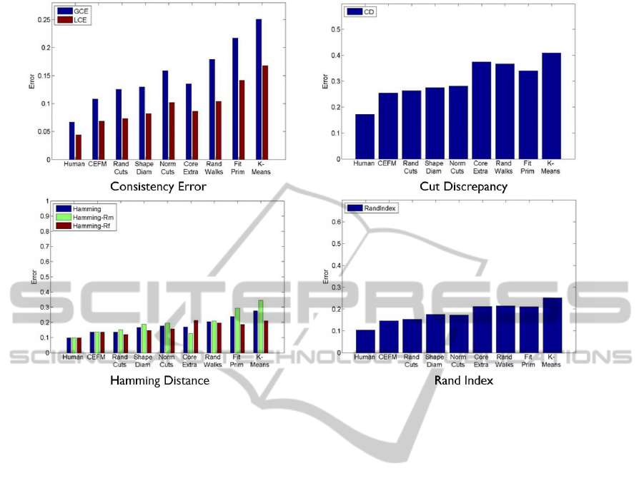
Figure 9: Evaluations using the performance measures proposed in (Chen et al., 2009) and the manual segmentations in the
Princeton Segmentation Benchmark. Our approach (short for ’CEFM’) clearly outperforms existing state-of-the-art automatic
segmentation approaches.
Until now, we have obtained a final segmentation
result, as shown in Fig.3(e). Note that the whole seg-
mentation procedure is completely automatic.
4 RESULTS
We have applied our method to segment a wide range
of models, including the whole set of models in
the Princeton Segmentation Benchmark (Chen et al.,
2009). As shown in our experiments, for most of
the models, the proposed approach is able to gener-
ate boundary cuts that adhere to the natural seams of
the models.
All 19 categories of 380 models in Princeton Seg-
mentation Benchmark were tested by our method.
As we can see from Fig.1, most segmentation re-
sults are satisfactory, especially for those models with
obvious salient parts, such as ants, bears, airplane,
and etc. We evaluated the segmentation results us-
ing the proposed metric methods in (Chen et al.,
2009). Fig.9 presents the quantitative results of our
method and other automatic segmentation methods.
Clearly, our easily-implemented and efficient method
outperforms existing state-of-the-art methods, includ-
ing complex methods like randomized cuts (Golovin-
skiy and Funkhouser, 2008). As shown in the bot-
tom left of Fig.9, the Hamming Distance of missing
rate (R
m
) of our method is lower while false alarm
rate (R
f
) is higher compared with randomized cuts
method. This is because our approach tends to seg-
ment shapes into more parts due to the heuristic strat-
egy. In terms of computation complexity, our ap-
proach is quite efficient and feasible. For a typical
model consisting of 10K triangles, the time needed
for a total computation process is less than 15 seconds
on an Intel 2.3GHz laptop with 4GB memory (codes
were written in Matlab under Windows 7).
However, there also exist several drawbacks in our
approach. Firstly, our method is not able to deal with
shapes containing inadequate or too similar volumet-
ric information, see Fig.10(a). This is because the
SDF descriptor has difficulty in distinguishing sepa-
rated parts of these shapes when detecting diameters
inside the shapes. Another drawback is that the re-
sults tend to be over-segmented if the shapes contain
a lot of folds on their surfaces (Fig.10(b)). Finally, for
certain models, the boundaries between segment parts
are not smooth enough and look unnatural, as shown
in Fig.10(c).
GRAPP2015-InternationalConferenceonComputerGraphicsTheoryandApplications
120
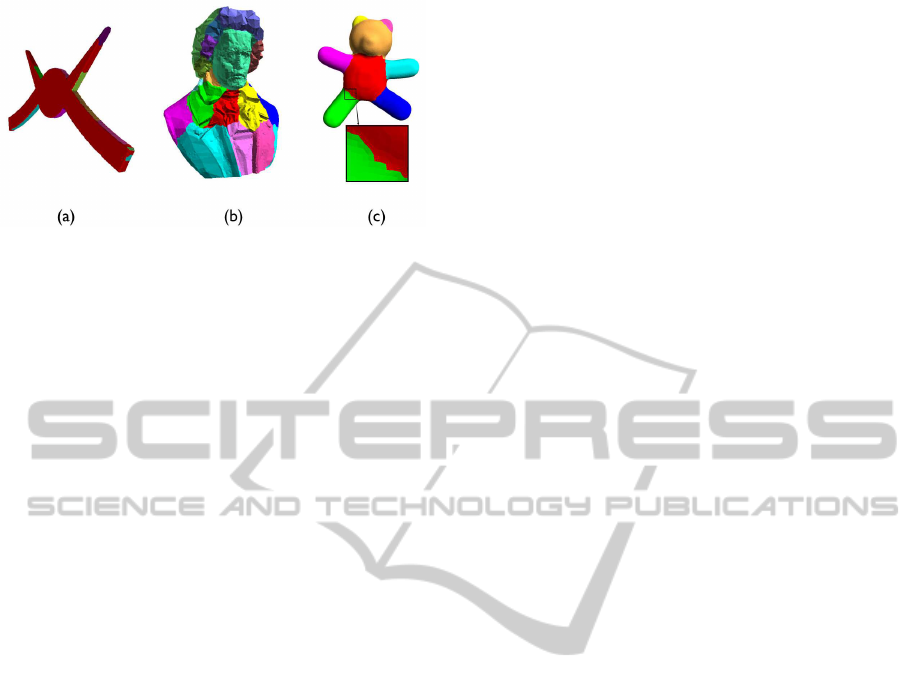
Figure 10: Limitations of our approach. (a) A sheet-like
plier model from SHREC’11(Lian et al., 2011) which is
hard to be segmented. (b) A bust model with lots of details.
(c) A bear model segmented with coarse boundaries.
5 CONCLUSION
In this paper, we introduced an efficient and effective
automatic mesh segmentation method based on the
detection of concave areas and heuristic 2-category
classification via fast marching. We demonstrated
the effectiveness of our method by carrying out seg-
mentation experiments on the Princeton segmentation
benchmark. Experimental results indicate that our
method clearly outperforms existing state-of-the-art
approaches in mesh segmentation.
ACKNOWLEDGEMENT
This work was supported by National Natural Sci-
ence Foundation of China (Grant No.: 61202230 and
61472015), National Hi-Tech Research and Develop-
ment Program (863 Program) of China (Grant No.:
2014AA015102).
REFERENCES
Bilmes, J. A. (1997). A gentle tutorial on the em algorithm
and its application to parameter estimation for gaus-
sian mixture and hidden markov models.
Boykov, Y., Veksler, O., and Zabih, R. (2001). Fast ap-
proximate energy minimization via graph cuts. IEEE
Transactions on Pattern Analysis and Machine Intel-
ligence, 23(11):1222–1239.
Chen, X., Golovinskiy, A., and Funkhouser, T. (2009). A
benchmark for 3D mesh segmentation. ACM Trans-
actions on Graphics, 28(3):Article No. 73.
Golovinskiy, A. and Funkhouser, T. (2008). Randomized
cuts for 3D mesh analysis. ACM Transactions on
Graphics, 27(5).
Kalogerakis, E., Hertzmann, A., and Singh, K. (2010).
Learning 3D mesh segmentation and labeling. ACM
Transactions on Graphics, 29(3):1–11.
Katz, S., Leifman, G., and Tal, A. (2003). Hierarchical
mesh decomposition using fuzzy clustering and cuts.
ACM Trans. Graphics, 22:954–961.
Katz, S., Leifman, G., and Tal, A. (2005). Mesh segmen-
tation using feature point and core extraction. The Vi-
sual Computer, 21(8):649–658.
Lai, Y., Hu, S., Martin, R. R., and Rosin, P. L. (2008). Fast
mesh segmentation using random walks. In Proceed-
ings of ACM symposium on Solid and Physical Mod-
eling, pages 183–191.
Lian, Z., Godil, A., Bustos, B., Daoudi, M., Hermans, J.,
Kawamura, S., Kurita, Y., Lavou, G., Nguyen, H.,
Ohbuchi, R., Ohkita, Y., Ohishi, Y., Porikli, F., Reuter,
M., Sipiran, I., Smeets, D., Suetens, P., Tabia, H., and
Vandermeulen, D. (2011). Shrec11 track: Shape re-
trieval on non-rigid 3d watertight meshes. Eurograph-
ics Workshop on 3D Object Retrieval.
Lin, J., Yang, Y., Lu, T., He, G., and Ruan, J. (2010). Mesh
segmentation by local depth. 2010 Second Interna-
tional Conference on Computer Modeling and Simu-
lation.
Liu, R. and Zhang, H. (2007). Mesh segmentation via
spectral embedding and contour analysis. In Com-
puter Graphics Forum (Special Issue of Eurographics
2007). Blackwell Publishing.
Sethian, J. (1999). Level Set Methods and Fast Marching
Methods Evolving Interfaces in Computational Geom-
etry, Fluid Mechanics, Computer Vision, and Materi-
als Science. Cambridge University Press, London, 1st
edition.
Shapira, L., Shalom, S., Shamir, A., Cohen-Or, D., and
Zhang, H. (2010). Contextual part analogies in 3d ob-
jects. International Journal of Computer Vision, pages
309–326.
Shapira, L., Shamir, A., and Cohen-Or, D. (2008). Con-
sistent mesh partitioning and skeletonisation using
the shape diameter function. The Visual Computer,
24(4):249–259.
Shlafman, S., Tal, A., and Katz, S. (2002). Metamorpho-
sis of polyhedral surfaces using decomposition. Com-
puter Graphics Forum, 21(3):219–228.
Zhang, H. and Liu, R. (2005). Mesh segmentation via re-
cursive and visually salient spectral cuts. In Proc. of
Vision, Modeling, and Visualization. VMV.
CEFM-AHeuristicMeshSegmentationMethodbasedonConvexityEstimationandFastMarching
121
