
Fractal Image Compression using Hierarchical Classification of
Sub-images
Nilavra Bhattacharya
1
, Swalpa Kumar Roy
1
, Utpal Nandi
2
and Soumitro Banerjee
3
1
Dept. of Computer Sc.& Tech., Indian Institute of Engineering Science & Technology, Shibpur, India
2
Dept. of Computer Science, Vidyasagar University, Midnapore, India
3
Dept. of Physical Sciences, Indian Institute of Science Education and Research, Kolkata, India
Keywords:
Fractal Image Compression, Fisher Classification, IFS, PIFS, Hierarchical Classification, Block Classification.
Abstract:
In fractal image compression (FIC) an image is divided into sub-images (domains and ranges), and a range
is compared with all possible domains for similarity matching. However this process is extremely time-
consuming. In this paper, a novel sub-image classification scheme is proposed to speed up the compression
process. The proposed scheme partitions the domain pool hierarchically, and a range is compared to only those
domains which belong to the same hierarchical group as the range. Experiments on standard images show that
the proposed scheme exponentially reduces the compression time when compared to baseline fractal image
compression (BFIC), and is comparable to other sub-image classification schemes proposed till date. The
proposed scheme can compress Lenna (512x512x8) in 1.371 seconds, with 30.6 dB PSNR decoding quality
(140x faster than BFIC), without compromising compression ratio and decoded image quality.
1 INTRODUCTION
The theory of fractal based image compression us-
ing iterated function system (IFS) was first proposed
by Michael Barnsley (Barnsley, 1988). A fully auto-
mated version of the compression algorithm was first
developed by Arnaud Jaquin, using partitioned IFS
(PIFS) (Jacquin, 1992). Jaquin’s FIC scheme is called
the baseline fractal image compression (BFIC). Frac-
tal compression is an asymmetric process. Encod-
ing time is much greater compared to decoding time,
since the encoding algorithm has to repeatedly com-
pare a large number of domains with each range to
find the best-match.
Plenty of research has focused on how to speed-
up the compression process, and almost all of them
explored how to reduce the number of domain blocks
in the domain pool. Fisher (1994) divided the domain
pool into 72 classes according to certain combinations
of the four quadrants of a block. His work proved the
efficiency of the classification schemes: the searching
time got reduced to the order of magnitude of sec-
onds without great loss of image quality. Tong and Pi
(2001) and later Wu et al. (2005) used standard devi-
ation to classify blocks. Wang et al. (2000) and Duh
et al. (2005) used the edge properties of the blocks to
group them into three or four classes, and this resulted
in a speedup ratio of 3 to 4. Xing et al. (2008) re-
fined Fisher’s scheme and obtained 576 classes based
on a block’s mean pixel value and its variance. Han
(2008) used a fuzzy pattern classifier to classify im-
age blocks. Tseng et al. (2008) used Particle Swarm
Optimization to classify image blocks. Jayamohan
and Revathy (2012) classified domains based on Lo-
cal Fractal Dimensions and used AVL trees to store
the classification. Wang and Zheng (2013) used Pear-
son’s Correlation Coefficient as a measure of similar-
ity between domains and ranges, and classified image
blocks based on it.
In this paper a novel sub-image classification
scheme is proposed, which greatly improves the com-
pression time (when compared to BFIC), and is com-
parable to other sub-image classification schemes
proposed till date, in terms of speed. The layout
of this paper is as follows: the mathematical back-
ground of Fractal Image Compression is briefly out-
lined in section 2, while Fisher’s classification scheme
is explained in section 3. The proposed classification
scheme (abbreviated as P-I) is explained in section 4.1
and a further optimization technique (abbreviated as
P-II) is given in section 4.2. Experimental results are
given in section 5. The conclusions are made in sec-
tion 6, which are followed by acknowledgements, and
finally the references.
46
Bhattacharya N., Roy S., Nandi U. and Banerjee S..
Fractal Image Compression using Hierarchical Classification of Sub-images.
DOI: 10.5220/0005265900460053
In Proceedings of the 10th International Conference on Computer Vision Theory and Applications (VISAPP-2015), pages 46-53
ISBN: 978-989-758-089-5
Copyright
c
2015 SCITEPRESS (Science and Technology Publications, Lda.)

2 FRACTAL COMPRESSION
2.1 The Theory
A typical affine transform from a domain to a range
is shown in Equation (1). Constants a
i, j
represent the
scaling factors from the domain to the range, while
constants d
i, j
represent the top-left corner of the do-
main. Constants s
i
and o
i
control the contrast and the
brightness of the transformation respectively. Hence,
an affine map is basically a collection of constants.
W
i
x
y
z
=
a
i,1
a
i,2
0
a
i,3
a
i,4
0
0 0 s
i
x
y
z
+
d
i,1
d
i,2
o
i
(1)
A domain and a range is compared using an RMS
metric (Fisher, 1994). Given two square sub-images
containing n pixel intensities, a
1
, . . . , a
n
(from the do-
main) and b
1
, . . . , b
n
(from the range), with contrast
s and brightness o between them, the RMS distance
between the domain and the range is given by
R =
n
∑
i=1
(s · a
i
+ o − b
i
)
2
(2)
Detailed mathematical description of IFS theory
and other relevant results can be found in (Barnsley,
1988; Edgar, 2007; Falconer, 2013).
2.2 The Pain
As mentioned in section 1, an enormous number of
domain-range comparisons is the main bottleneck of
the compression algorithm. E.g., consider an image
of size 512 × 512. Let the image be partitioned into
4 × 4 non-overlapping range blocks. There will be
2
14
= 16384 range blocks. Let there be 8×8 overlap-
ping domain blocks (most implementations use do-
main sizes that are double the size of range). Then, for
a complete search, each range block has to be com-
pared with 505 × 505 = 255025 domain blocks. The
total number of comparisons will be around 2
32
. The
time complexity can be estimated as Ω(2
n
).
3 FISHER’S CLASSIFICATION
Fisher’s classification scheme (Fisher, 1994) is as
follows: A square sub-image (domain or range) is
divided into upper-left, upper-right, lower-left, and
lower-right quadrants, numbered sequentially.
On each quadrant, values A
i
(proportional to mean
pixel intensity) and V
i
(proportional to pixel intensity
variance) are computed. If the pixel values in quad-
rant i are r
i
1
, r
i
2
, . . . , r
i
n
, then
A
i
=
n
∑
j=1
r
i
j
(3)
and
V
i
=
n
∑
j=1
(r
i
j
)
2
− A
2
i
(4)
Then it is possible to rotate the sub-image (do-
main or range) such that the A
i
are ordered in one of
the following three ways:
Major Class 1: A
1
≥ A
2
≥ A
3
≥ A
4
Major Class 2: A
1
≥ A
2
≥ A
4
≥ A
3
Major Class 3: A
1
≥ A
4
≥ A
2
≥ A
3
These orderings constitute three major classes and
are called canonical orderings. Under each major
class, there are 24 subclasses consisting of
4
P
4
= 24
orderings of the V
i
. Thus there are 72 classes in all.
Fisher noted that the distribution of domains across
the 72 classes was far from uniform. So he went on
to further simplify the scheme. 24 classes were de-
rived by combining the three major first-classes in the
above classification. Fisher concluded: ”the improve-
ment attained by using 72 rather than 24 classes is
minimal and comes at great expense of time” (Fisher,
1994). In this paper, we refer to this 24-class classifi-
cation scheme as FISHER24.
4 PROPOSED HIERARCHICAL
CLASSIFICATION SCHEME
Fisher used values proportional to the mean and the
variance of the pixel intensities to classify a sub-
image. In our proposed schemes, we use only the sum
of pixel intensities of various parts of a sub-image to
classify the sub-image.
4.1 Proposed Technique - I (P-I)
After selecting the square sub-image (domain / range)
(Figure 1(a)), the proposed hierarchical classification
algorithm works as follows:
1. Divide the sub-image into upper-left, upper-right,
lower-left, and lower-right quadrants.
2. For each quadrant i (i = 0, 1, 2, 3) calculate the
sum of pixel values S
i
. If the pixel values in quad-
rant i are r
i
1
, r
i
2
, . . . , r
i
n
, then
S
i
=
n
∑
j=1
r
i
j
(5)
FractalImageCompressionusingHierarchicalClassificationofSub-images
47
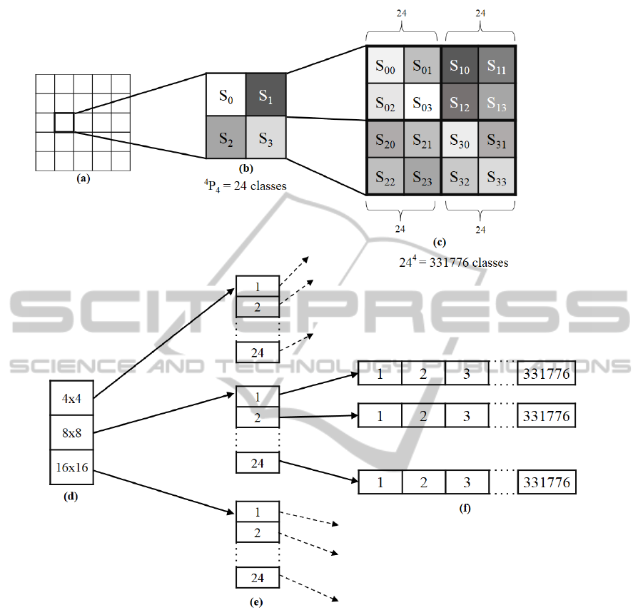
Figure 1: Proposed classification scheme and data structures used: (a) Square sub-images (overlapping domains or non-
overlapping ranges) (b) Level I classification - 24 classes based on relative ordering of pixel intensity sums S
0
, S
1
, S
2
, S
3
(c)
Level II classification - 4 quadrants of Level I further subdivided into 4 sub-quadrants each; each quadrant i assigned a value
between 1 and 24 based on relative ordering of sub-quadrant pixel intensity sums S
i0
, S
i1
, S
i2
, S
i3
(i = 0, 1, 2, 3). 4 quadrants,
each having a value between 1 and 24 gives 3311776 classes. (d) Domain pool has domains of 3 sizes - 4 × 4, 8 × 8 and
16 × 16 (e) 24 Level I classes for all 3 domain sizes (f) 331776 Level II classes for every Level I class. Each of the 331776
array cells point to a list of domains falling in that class.
3. Based on the relative ordering of S
0
, S
1
, S
2
, S
3
(calculated in Step 2), there can be
4
P
4
= 24 per-
mutations. A number between 1 and 24, that
uniquely identifies this particular permutation is
assigned to this sub-image. This number is the
Level I class for this sub-image (Figure 1(b)).
4. Divide each of the quadrants of Step 1 again, into
4 sub-quadrants (16 sub-quadrants in total).
5. Calculate the sum of pixel values S
i j
(i =
0, 1, 2, 3, j = 0, 1, 2, 3) for each sub-quadrant.
6. Based on the relative ordering of sub-quadrant
pixel-value sums S
i0
, S
i1
, S
i2
, S
i3
for each quad-
rant i = 0, 1, 2, 3, each quadrant can be assigned
a number between 1 and 24 (similar to step 3).
Four quadrants, each being assigned a number be-
tween 1 and 24 gives 24
4
= 331776 cases in to-
tal, for the entire sub-image. A number between 1
and 331776, that uniquely identifies this particular
case is assigned to this sub-image. This number is
the Level II class for this sub-image (Figure 1(c)).
VISAPP2015-InternationalConferenceonComputerVisionTheoryandApplications
48

During compression, when the domain pool is be-
ing created, data structures are defined as shown in
Figure 1(d), Figure 1(e) and Figure 1(f). Domains
are first classified by their size, then into Level-I, ac-
cording to pixel-value-sum of 4 quadrants, and finally
into Level-II, according to pixel-value sum of 16 sub-
quadrants. After two rounds of classification, the do-
main is placed in a list pointed to by the array cell
corresponding to the Level-II class (Figure 1(f)).
Later in the compression algorithm, when search-
ing the domain pool for a best-match with a particular
range, only those domains that are in the same Level-
II class as the range are considered for comparison.
4.2 Proposed Technique - II (P-II)
This is an add-on for the proposed P-I technique (sec-
tion 4.1) to further reduce the number of domain-
range comparisons. The main idea is to keep track of
the domains that are getting selected as the best-match
more than once, and offering those domains for com-
parison in subsequent searches, before others, hoping
that these will again be a best-match, and searching
will be over quickly. This is implemented as follows:
Along with each domain, a counter named
timesUsed is also maintained, which indicates how
many times that particular domain was already se-
lected as the best-match. During the creation of
the domain pool, all timesUsed counters of all do-
mains are initialized to zero. Later, when search-
ing the domain-list of a Level-II class for the best-
match, if a domain gets selected as the best-match, its
timesUsed counter value is incremented.
On subsequent searches in the same Level-II class,
domains are selected for comparison in the decreasing
order of their timesUsed value. Searching gets over
as soon as a domain is found whose RMS distance
from the range is less than a predefined threshold.
Once again the timesUsed value of this best-match
domain is incremented.
The domain-lists of each Level-II class are imple-
mented as max-heaps which support O(logn) time in-
serts and O(1) lookups (Cormen et al., 2009).
4.3 Elementary Analysis
4.3.1 FISHER24
Let total number of domains in domain-pool = D
Number of classes = 24
∴ Average number of domains per class =
D
24
Let total number of ranges = R
∴ Number of domain-range comparisons =
D
24
· R (6)
4.3.2 P-I
Let total number of domains in domain-pool = D
Number of Level-I classes = 24
Number of Level-II classes = 24
4
∴ Total number of classes = 24 · 24
4
= 24
5
∴ Average number of domains per class =
D
24
5
Let total number of ranges = R
∴ Number of domain-range comparisons =
D
24
5
· R (7)
4.3.3 P-II
Let total number of domains in domain-pool = D
Number of Level-I classes = 24
Number of Level-II classes = 24
4
∴ Total number of classes = 24 · 24
4
= 24
5
∴ Average number of domains per class =
D
24
5
Let total number of ranges = R
∴ Number of domain-range comparisons
≤
D
24
5
· R (8)
In Equation (8), the less-than condition occurs be-
cause searching is over as soon as a domain is found
whose RMS distance from the range is less than the
predefined threshold. Equality occurs in the worst-
case, when only the last domain of a class is selected
every time.
It is evident from the above analysis that since
D
24
5
· R
D
24
(9)
the proposed classification schemes reduce the do-
main search space exponentially, when compared to
FISHER24. This is bound to speed up the compres-
sion algorithm, and is corroborated by the experimen-
tal results in section 5.
FractalImageCompressionusingHierarchicalClassificationofSub-images
49
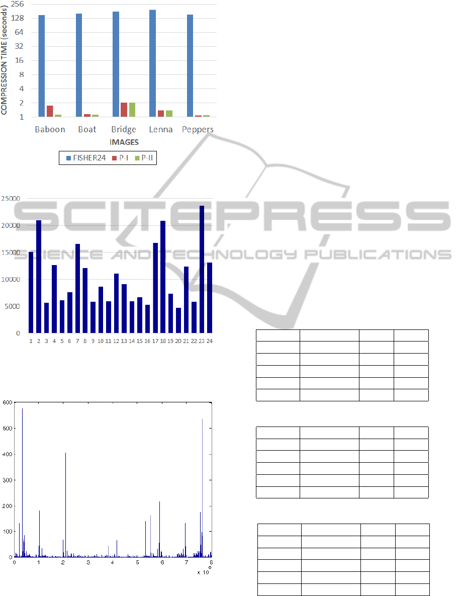
Figure 2: Graphical comparison of compression time.
Figure 3: Histogram of ”Lenna” showing the number of do-
mains in each of the 24 classes of FISHER24 classification
scheme (summed across all the domain sizes).
Figure 4: Histogram of ”Lenna” showing the number of
domains in each of the 24
5
classes of the proposed classifi-
cation scheme (summed across all the domain sizes).
5 RESULTS AND DISCUSSIONS
5.1 Tools
Five standard 512 × 512 × 8 images have been used to
test the proposed techniques P-I (section 4.1) and P-II
(section 4.2) and also for comparison with FISHER24
classification scheme (section 3). The algorithm was
implemented in Java, running on a PC with Intel Core
i7 2630QM 2.0 GHz Processor, 8 GB DDR3 RAM,
and running Windows 8 x64.
5.2 Research Results
The comparison of compression time (in seconds),
PSNRs (in dB) and space savings (in percentage) for
the five image files have been made in Table 1, Table 2
and Table 3 respectively. The pictorial representations
of compression times, PSNRs and space savings are
illustrated in Figures 2, 5 and 6 respectively. Figures
7, 8, 9 and 10 show the close up of Lenna original,
decoded after using FISHER24, decoded after using
proposed P-I technique and decoded after using pro-
posed P-II technique respectively. Figure 11 shows
the result of the techniques on the other test images.
Table 1: Comparison of compression time (seconds).
Image FISHER24 P-I P-II
Baboon 147.441 1.737 1.137
Boat 160.214 1.161 1.133
Bridge 175.924 2.035 1.995
Lenna 193.066 1.371 1.374
Peppers 150.112 1.082 1.102
Table 2: Comparison of PSNR (in dB).
Image FISHER24 P-I P-II
Baboon 22.22 22.22 22.22
Boat 28.44 28.44 28.44
Bridge 25.55 25.55 25.56
Lenna 30.60 30.60 30.60
Peppers 28.01 28.01 28.02
Table 3: Comparison of Space Savings (%).
Image FISHER24 P-I P-II
Baboon 89.26 89.26 89.26
Boat 89.39 89.39 89.39
Bridge 86.88 86.88 86.88
Lenna 89.58 89.58 89.58
Peppers 89.43 89.43 89.43
The proposed two techniques exponentially re-
duce the compression time compared to FISHER24.
VISAPP2015-InternationalConferenceonComputerVisionTheoryandApplications
50
It is because the total number of domain-range com-
parisons is reduced, as shown by Equation (9).
Figures 3 and 4 show the distribution of domains
across all classes for FISHER24 and the proposed
classification scheme respectively, for the Lenna im-
age. Figure 3 shows that each class contains at least
5000 domains. So each range is compared to a mini-
mum of 5000 domains. However, Figure 4 shows that
in the proposed scheme, most classes contain less than
100 domains, while the maximum number domains
in a class is less than 600. So the total number of
domain-range comparisons is greatly reduced in the
proposed schemes. Between the two proposed tech-
niques, P-II takes less time for 3 out of 5 test-images.
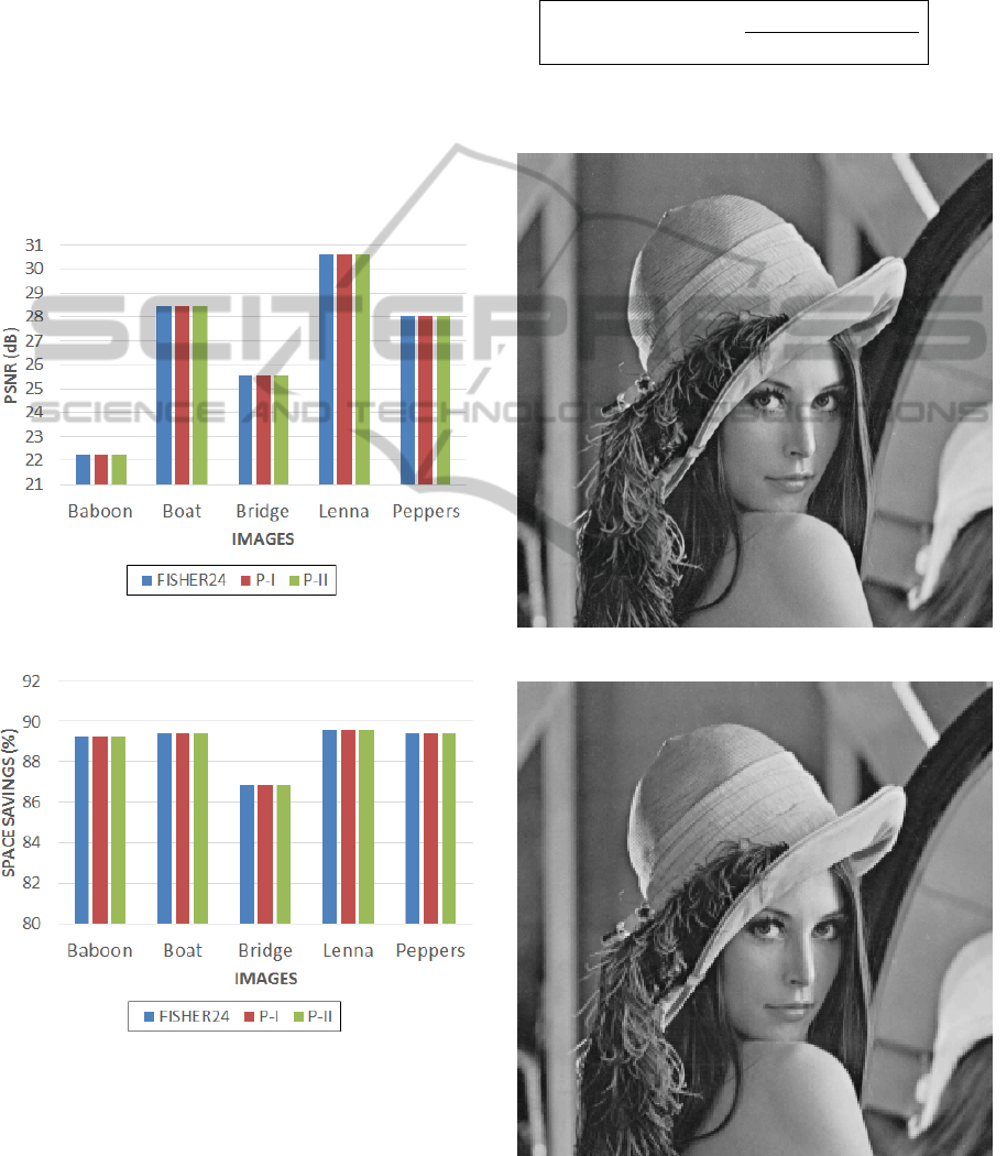
Figure 5: Graphical comparison of PSNR.
Figure 6: Graphical comparison of Space Savings (%).
Regarding decoded image quality, Table 2 and
Figure 5 shows that the proposed techniques offer the
same quality as FISHER24, for all the test-images.
The PSNR values are identical for all the recon-
structed images, even for P-II, where the search is
being terminated as soon as a domain with domain-
range RMS distance less than a predefined threshold
is found. This means that the best domains are being
used maximum number of times.
Space Savings is the reduction in size relative to
uncompressed size, and is given as
Space Savings = 1 −
Compressed Size
Uncompressed Size
(10)
The proposed two techniques offer almost the
same percentage of space-savings as FISHER24.
Figure 7: Lenna - original.
Figure 8: Lenna - using FISHER24 classification.
FractalImageCompressionusingHierarchicalClassificationofSub-images
51

Figure 9: Lenna - after using proposed technique P-I.
Figure 10: Lenna - after using proposed technique P-II.
6 CONCLUSION
The proposed techniques of Fractal Image Com-
pression by using hierarchical classification of do-
main/range viz. P-I and P-II improve the compres-
sion time of images significantly, when compared
to existing FISHER24 classification. PSNRs of de-
coded images using both techniques are identical to
FISHER24, which means that image quality is not
degraded by the proposed techniques. The compres-
sion ratios (denoted by space savings in this paper)
for both P-I and P-II are also equal to FISHER24. Be-
tween the two proposed techniques, P-II is marginally
faster than P-I in 3 out of 5 test-images. In terms of
PSNR and space savings, they give identical results.
ACKNOWLEDGEMENTS
The first author acknowledges the support of the
AICTE-INAE Travel Grant Scheme for Engineering
Students, Govt. of India, which enabled him to attend
the conference.
The first-author also thanks the German Missions
in India for offering a free Schengen VISA to attend
the conference.
REFERENCES
Barnsley, M. F. (1988). Fractals Everywhere. Academic
Press, New York.
Cormen, T. H., Leiserson, C. E., Rivest, R. L., and Stein,
C. (2009). Introduction to Algorithms. MIT press,
Cambridge, MA, U.S.A.
Duh, D.-J., Jeng, J., and Chen, S.-Y. (2005). Dct based sim-
ple classification scheme for fractal image compres-
sion. Image and vision computing, 23(13):1115–1121.
Edgar, G. (2007). Measure, topology, and fractal geometry.
Springer.
Falconer, K. (2013). Fractal geometry: mathematical foun-
dations and applications. John Wiley & Sons.
Fisher, Y., editor (1994). Fractal Image Compression: The-
ory and Application. Springer-Verlag, New York.
Han, J. (2008). Fast fractal image compression using fuzzy
classification. In Fuzzy Systems and Knowledge Dis-
covery, 2008. FSKD’08. Fifth International Confer-
ence on, volume 3, pages 272–276. IEEE.
Jacquin, A. E. (1992). Image coding based on a fractal the-
ory of iterated contractive image transformations. Im-
age Processing, IEEE Transactions on, 1(1):18–30.
Jayamohan, M. and Revathy, K. (2012). An improved do-
main classification scheme based on local fractal di-
mension. Indian Journal of Computer Science and
Engineering (IJCSE), 3(1):138–145.
Tong, C. S. and Pi, M. (2001). Fast fractal image encoding
based on adaptive search. Image Processing, IEEE
Transactions on, 10(9):1269–1277.
Tseng, C.-C., Hsieh, J.-G., and Jeng, J.-H. (2008). Frac-
tal image compression using visual-based particle
swarm optimization. Image and Vision Computing,
26(8):1154–1162.
Wang, J. and Zheng, N. (2013). A novel fractal image com-
pression scheme with block classification and sorting
based on pearson’s correlation coefficient.
Wang, Z., Zhang, D., and Yu, Y. (2000). Hybrid image
coding based on partial fractal mapping. Signal Pro-
cessing: Image Communication, 15(9):767–779.
VISAPP2015-InternationalConferenceonComputerVisionTheoryandApplications
52
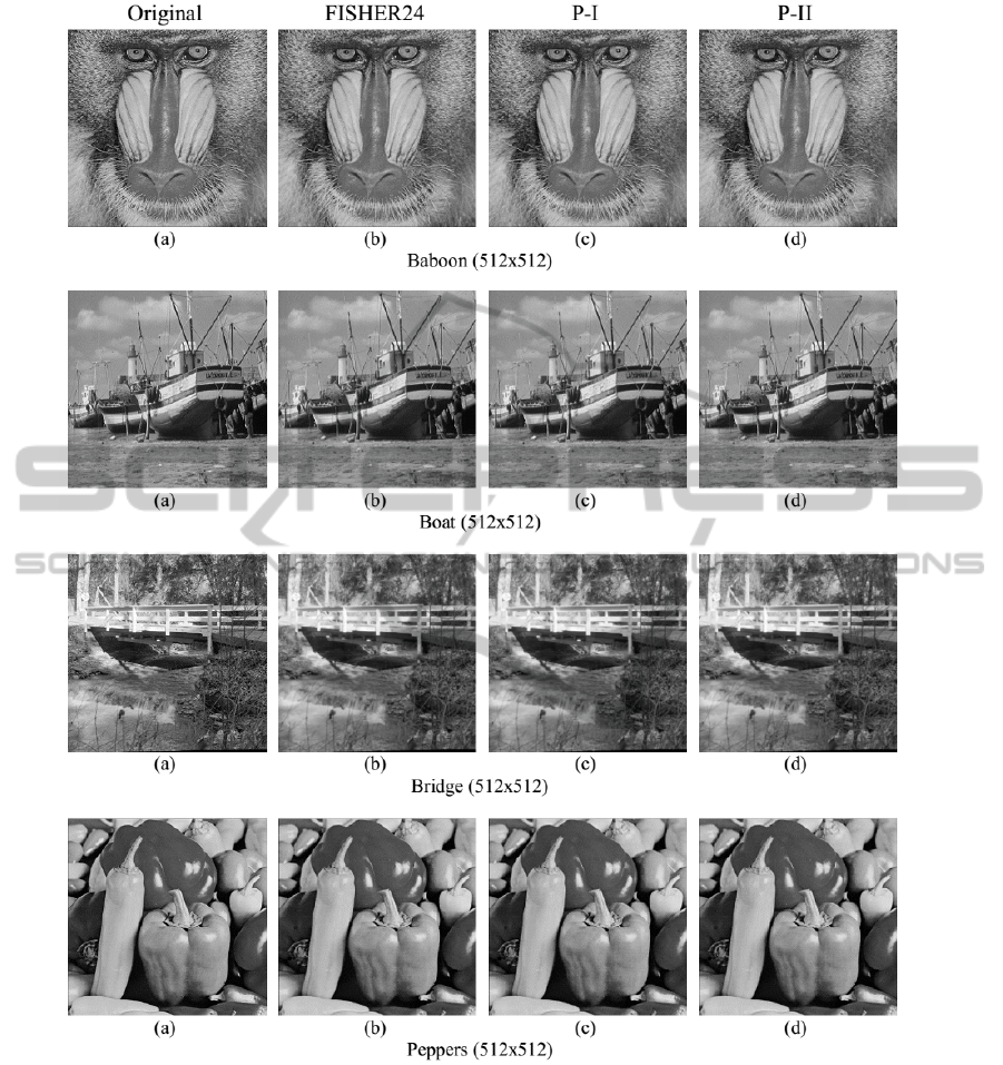
Figure 11: Test images and results - Baboon, Boat, Bridge and Peppers. (a) Original image (b) Result of using FISHER24
classification (c) Result of using proposed P-I technique (d) Result of using proposed P-II technique.
Wu, X., Jackson, D. J., and Chen, H.-C. (2005). A fast frac-
tal image encoding method based on intelligent search
of standard deviation. Computers & Electrical Engi-
neering, 31(6):402–421.
Xing, C., Ren, Y., and Li, X. (2008). A hierarchical classi-
fication matching scheme for fractal image compres-
sion. In Image and Signal Processing, 2008. CISP’08.
Congress on, volume 1, pages 283–286. IEEE.
FractalImageCompressionusingHierarchicalClassificationofSub-images
53
