
High-Speed and Robust Monocular Tracking
Henning Tjaden
1
, Ulrich Schwanecke
1
, Fr
´
ed
´
eric A. Stein
2
and Elmar Sch
¨
omer
2
1
Computer Science Department, RheinMain University of Applied Science, Unter den Eichen 5, Wiesbaden, Germany
2
Institute of Computer Science, Johannes-Gutenberg University, Staudingerweg 9, Mainz, Germany
Keywords:
Optical Tracking, Monocular Pose Estimation System, Infrared LED, Camera, High-Speed, Calibration.
Abstract:
In this paper, we present a system for high-speed robust monocular tracking (HSRM-Tracking) of active
markers. The proposed algorithm robustly and accurately tracks multiple markers at full framerate of current
high-speed cameras. For this, we have developed a novel, nearly co-planar marker pattern that can be identified
without initialization or incremental tracking. The pattern also encodes a unique ID to identify different
markers. The individual markers are calibrated semi-automatically, thus no time-consuming and error-prone
manual measurement is needed. Finally we show that the minimal spatial structure of the marker can be used
to robustly avoid pose ambiguities even at large distances to the camera. This allows us to measure the pose
of each individual marker with high accuracy in a vast area.
1 INTRODUCTION AND
BACKGROUND
Tracking of moving objects is a very important aspect
in many fields of application such as robotics, auto-
motive, sports, health, or virtual reality. Often it is
the basis to automatically supervise, classify and op-
timize motion sequences such as in athletic training
or medical therapy (Fitzgerald et al., 2007; Vito et al.,
2014). Other applications can be found in industrial
assembly, where optical tracking can be used to assist
humans or robots in order to increase their productiv-
ity and reliability or enables them to work more au-
tonomously (Ong and Nee, 2004; Zetu et al., 2000).
Over the past decades, a large number of different
solutions have been developed to track the position
and orientation of objects based on various technolo-
gies such as ultrasound, magnetism, inertial, or opti-
cal sensors (Welch and Foxlin, 2002). Most widely
used are probably the optical tracking systems which
can be divided into active and passive systems. Pas-
sive systems use just the visible light to detect high
contrast artificial fiducials or natural structures. Ac-
tive systems use additional light sources to facilitate
the detection of specially designed fiducials. Thereby,
they usually work with infrared light to minimize the
influence of ambient lighting.
Active optical tracking systems can be divided fur-
ther into systems where the additional light source
is attached to the camera – also called active cam-
era systems – and systems with light emitting devices
such as light emitting diodes (LEDs) attached to the
fiducials – also called active tracker systems. While
active camera systems utilize very lightweight and
keen targets, active tracker systems usually provide
a larger total working volume and higher precision.
Optical tracking systems often determine the
three-dimensional position of a ball-like fiducial
based on two or more camera images and triangula-
tion. While this can be done very efficiently utilizing
epipolar constraints, it requires the fiducials always
to be seen by (at least) two cameras. In some applica-
tions, this may not always be guaranteed and a system
based on the image of just a single monocular camera
is needed. In this work we therefore focus on tracking
with a single monocular optical camera.
In its simplest form, optical tracking of the pose of
a rigid object with a single camera is based on passive
planar markers (Olson, 2011; Herout et al., 2013).
The advantage of these passive systems is their low
complexity. Users can simply print or even draw their
own markers. But, even though the latest methods
achieve higher robustness against fast movement by
tracking arbitrary patterns based on feature descrip-
tors (Wagner et al., 2008; Ozuysal et al., 2010), or
using a parametrized model of the object under inves-
tigation (Schmaltz et al., 2012; Prisacariu and Reid,
2012), passive systems are still limited in distance
range and stability under low lighting conditions or
lack in terms of precision or high-speed performance.
462
Tjaden H., Schwanecke U., Stein F. and Schömer E..
High-Speed and Robust Monocular Tracking.
DOI: 10.5220/0005267104620471
In Proceedings of the 10th International Conference on Computer Vision Theory and Applications (VISAPP-2015), pages 462-471
ISBN: 978-989-758-091-8
Copyright
c
2015 SCITEPRESS (Science and Technology Publications, Lda.)
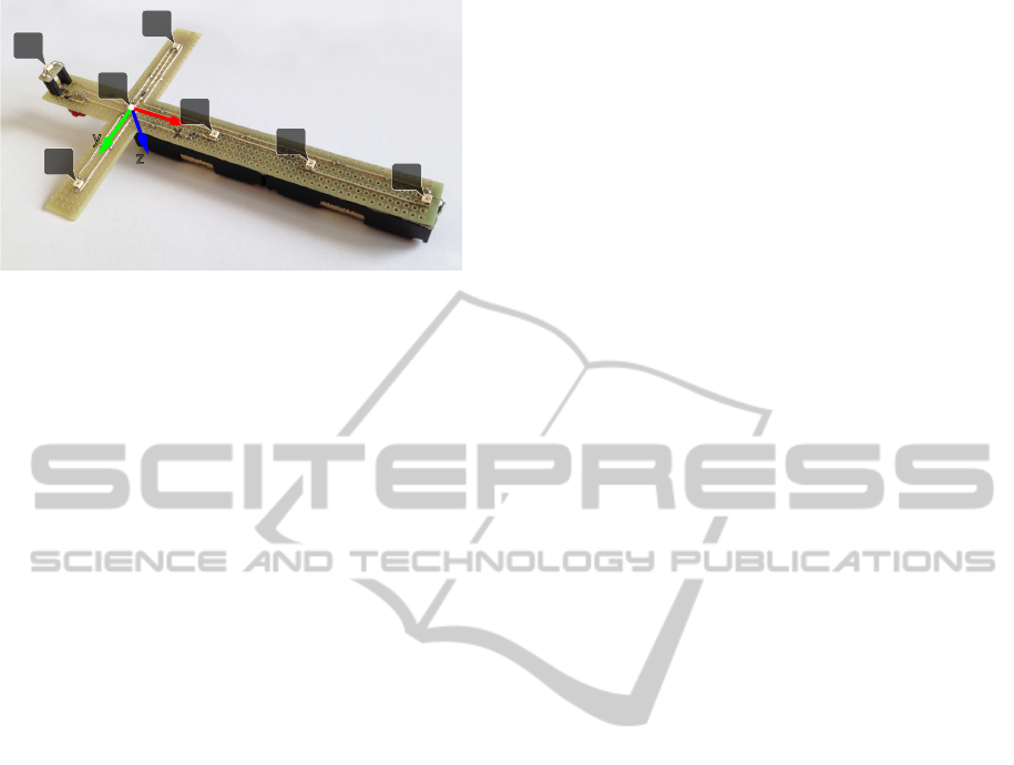
y
z
x
M4
M0
M1
M2
M3
M6
M5
Figure 1: The proposed markers consist of seven LEDs ar-
ranged in a cross-shaped pattern, where M
2
,M
3
,M
5
define
the right handed marker coordinate frame.
Active tracking systems overcome most of the
previously mentioned limitations as they are less de-
pendent on the given lighting conditions. One of
the main tasks of active systems is the identifica-
tion of the individual lights or retro-reflective tags
each marker is composed of. (Naimark and Foxlin,
2005) e.g. presented a technique for encoding indi-
vidual LED markers by amplitude modulation, used
in an initialization step. After initialization the LEDs
are tracked incrementally from frame to frame. Such
techniques come with the downside of potential track-
ing losses, after which the system would have to get
re-initialized.
Monocular tracking of purely co-planar markers
suffers from pose ambiguities, while markers with
spatial structure are likely to occlude themselves.
(Faessler et al., 2014) recently presented a system,
that can track a single marker composed of four or
five LEDs at 90 Hz. Although these LEDs can be ar-
ranged arbitrarily, they should span a volume as large
as possible to avoid pose ambiguities. The resulting
self-occlusions are dealt with a time consuming com-
binatorial brute force approach, that is used to ini-
tialize and re-initialize the LED identification. Once
initialized the LEDs are tracked incrementally in con-
junction with motion prediction. The spatial positions
of the marker LEDs are calibrated with a commercial
multi-camera motion capturing system.
In this paper we present a high-speed and robust
monocular (HSRM) tracking system that is superior
to all other present systems regarding accuracy, track-
ing range and robustness, while still being low-cost on
the hardware side. The system can estimate the pose
of multiple markers, each of them composed of seven
infrared LEDs, at frequencies far over 500 Hz, allow-
ing robust tracking even of fast-moving objects. Our
three main contributions are: First, a method to iden-
tify each individual LED of a marker solely based on
2D geometrical constraints not requiring any initial-
ization or frame-to-frame tracking. Second, an empir-
ical proof that the minimal 3D structure of our nearly
co-planar marker is an optimal tradeoff between the
occurrence of self-occlusions and the avoidance of
pose ambiguities. Third, a semi-automatic marker
calibration algorithm avoiding time-consuming and
error-prone manual measurements and ensuring accu-
rate tracking results.
2 MONOCULAR MARKER
TRACKING
In the following we describe our marker pattern and
its identification as well as the tracking of multiple
markers in detail. We also show that our approach
is robust to measurement noise and pose ambiguities
and present an algorithm to semi-automatically cali-
brate our markers with high accuracy.
2.1 Preliminaries
The proposed markers consist of seven infrared LEDs
connected to a small battery pack (Figure 1). For our
prototype we chose SMD (surface-mounted device)
LEDs which are perceptible from large viewing an-
gles up to nearly π/2. We tested our system with a
variety of monochrome USB 3.0 high-speed cameras,
operating from 90 Hz to 500 Hz with resolutions up to
2048×2048 pixels. The cameras have pre-calibrated
intrinsics and are equipped with an infrared filter to
reduce the influence of ambient light.
The marker LEDs are arranged in a constrained
geometrical cross-shaped pattern. The spatial LED
positions are denoted relative to the marker coordi-
nate frame and are referred to as M
i
= (x
i
,y
i
,z
i
)
>
,i =
0,.. .,6. Their corresponding 2D projections into
the camera image are denoted by m
i
= (x
i
,y
i
)
>
,i =
0,.. .,6. LED M
3
= (0,0, 0)
>
defines the origin of
the right handed marker coordinate frame, while the
vectors
−−−−→
M
3
M
2
and
−−−−→
M
3
M
5
define the corresponding
x- and y-axis, respectively. M
0
,.. .,M
5
lie in the xy-
plane and M
6
is slightly elevated for stabilization pur-
poses as will be explained in section 2.2.3. In sec-
tion 3 we show, that the exact spatial positions of all
LEDs can be measured automatically (up to a scaling
factor) in a pre-calibration step.
We refer to the pose of a marker with respect to
the camera coordinate frame as P
M
= [R
M
|t
M
], with
R
M
∈SO(3) describing the rotation of the marker and
t
M
∈R
3
being the location of the origin of the marker
coordinate frame in the camera coordinate frame. Per-
spective projection of a 3D point M including deho-
mogenisation is denoted by π(M) = (x/z,y/z)
>
.
High-SpeedandRobustMonocularTracking
463
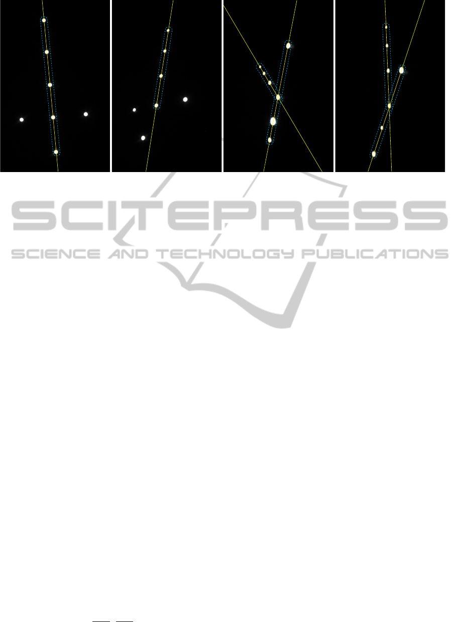
m0
m4
m5
m6
m3
m2
m1
l1
(a) Case L5.
m0
m4
m5
m6
m3
m2
m1
l1
(b) Case L41.
m0
m4
m5
m6
m3
m2
m1
l1
l2
(c) Case L42a.
m0
m4
m5
m6
m3
m2
m1
l1
l2
(d) Case L42b.
Figure 2: Raw input video frames of a marker under various perspective transformations showing the different configurations
distinguished during correspondence assignment. The dominant lines l
1
and l
2
are drawn and their participants are framed by
a dashed line. (a) An example where five LED projections lie on l
1
. (b) An example where l
1
has four participants. (c) An
example where two dominant lines appear in the projection pattern. In this case m
6
lies between m
4
and m
5
on l
2
. (d) The
second case where two dominant lines appear. In this case m
6
lies outside of m
4
and m
5
on l
2
.
2.2 Tracking Method
The pose of each marker is determined based on the
known 3D positions M
i
of the seven LEDs and their
corresponding 2D projections m
i
. Therefore, in a first
step we segment the projected LEDs in each video
frame and determine their exact 2D positions as ex-
plained in detail in section 2.2.1. After the 2D pro-
jections are segmented they have to be assigned to
the corresponding LEDs. Since all LED projections
look alike they cannot be distinguished by simple lo-
cal analysis. In section 2.2.2 we show how to deter-
mine the correct correspondences, while section 2.2.3
explains how to estimation the pose of the markers.
Finally, in section 2.2.4 the extension to multi-marker
tracking is presented.
2.2.1 LED Segmentation and 2D Localization
The LEDs will appear as bright blobs in the video
frames. These regions are saturated to a great extent
and therefore are significantly brighter than the rest
of the scene. To reduce the influence of ambient light,
we utilize an infrared filter, so that almost only the
LEDs remain visible in the camera image. To segment
the blobs, we use a simple binary thresholding, keep-
ing only pixels with an intensity above a prescribed
threshold s. The remaining pixels are grouped into
connected regions Ω
i
using a union-find algorithm.
In a next step we determine the 2D positions
m
0
i
=
m
10i
m
00i
,
m
01i
m
00i
>
(1)
of the LED projections by calculating the intensity
centroid of each region Ω
i
based on the moments
m
pqi
=
∑
(x,y)∈Ω
i
x
p
y
q
I(x,y)
2
. (2)
Thereby, we used a quadratic weighting of the pixel
intensities I(x, y) to reduce the influence of border
pixels, that tend to flicker due to their lower intensities
compared to pixels near the centroid. Experiments
showed that (2) reduces jitter of the measurements
similarly to applying a low-pass filter (e.g. Gaussian),
while being computationally less expensive.
In a last step all determined LED projections m
0
i
are normalized and undistorted to ideal image coordi-
nates m
i
using the pre-calibrated camera intrinsics.
2.2.2 Determining the 2D/3D Correspondences
Our constrained cross-shaped marker pattern allows
to determine the correspondences between 3D LED
position M
i
and ideal image coordinate m
i
for each
individual frame. Thereby, the only restriction is that
all seven LEDs of a marker have to be visible in the
respective frame.
Because m
0
,.. .,m
3
always must lie on a straight
line, we start by investigating the dominant lines in
the set of projections M = {m
0
,.. .,m
6
}. The first
dominant line l
1
can either have four participants
(case L4, see (Fig. 2(b)), five participants (case L5,
see Fig. 2(a)) or more than five participants. The lat-
ter case only occurs under very shallow viewing an-
gles with low measuring accuracy and will therefore
not be further considered.
VISAPP2015-InternationalConferenceonComputerVisionTheoryandApplications
464
Due to the structure of the marker there exist per-
spective transformations where m
6
together with m
3
,
m
4
and m
5
forms a second dominant line l
2
(see
Figs. 2(c) and 2(d)). Thus, case L4 is further sepa-
rated into L41 (one line) and case L42 (two lines).
These two cases can be differentiated based on re-
gression lines to all thirty-five subsets of four points
from M . Therefore, the lines and their correspond-
ing points are grouped by quality and angle, where
quality is determined by the distance of the furthest
outlier to the line. The cases L5, L41 and L42 now
can be distinguished as follows, based on simple 2D
geometric criteria:
L5: The two points that do not belong to l
1
define
a second line l
2
. The closest point to the inter-
section of l
1
and l
2
must be m
3
. The point that
lies solely on one side of l
2
is m
6
. The points
m
0
,m
1
,m
2
are assigned descendingly according
to their absolute distance to l
2
. Finally m
4
and m
5
are assigned based on their signed distance to the
line l
03
given by m
0
,m
3
.
L41: The point belonging to l
1
furthest from the cen-
troid of the three points not lying on l
1
must be
m
0
. Next, m
1
,m
2
and m
3
can be assigned ascend-
ingly according to their distance to m
0
. One of
the three remaining LEDs (either m
4
or m
5
) will
lie solely on one side of l
03
. It can be detected and
assigned by calculating the three signed distances
to l
03
. Assuming it is m
5
, we construct line l
35
given by m
3
,m
5
and assign m
4
and m
6
ascend-
ingly to their distance to it.
L42: We first identify l
1
by the fact that all points in-
cident to l
1
lie on the same side of line l
2
, except
m
3
which is the intersection of l
1
and l
2
. Next,
we can enumerate m
0
, m
1
and m
2
in descending
order according to their distance to m
3
. Now the
LED that lies solely on one side of l
1
is either m
4
or m
5
. Thereby the correct assignment is deter-
mined by the signed distance to l
1
as in L41. As-
suming that this assignment was m
5
, there are two
possibilities (L42a and L42b) to assign m
6
and
m
4
, which can not be robustly distinguished by
2D criteria (see Figs. 2(c) and 2(d)). We therefore
solve this ambiguity with regard to the 3D struc-
ture of the marker. This is done by calculating the
two homographies H
46
and H
64
for both possible
assignments from all six coplanar LEDs. These
homographies allow us to calculate two pose esti-
mations (Xu et al., 2009) called P
H46
and P
H64
.
To determine the correct assignment, we calcu-
late the average reprojection errors (see eqn. (3)
in section 2.2.3) for both pose estimations using
all seven LEDs and choose the assignment com-
bination that yields the smaller error.
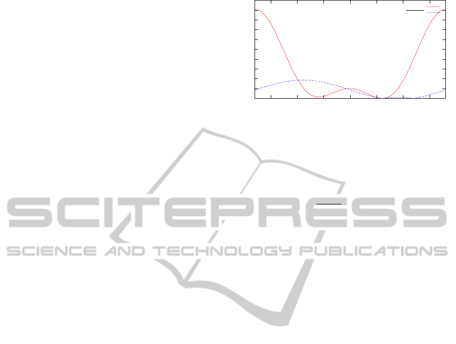
0
0.01
0.02
0.03
0.04
0.05
0.06
0.07
0.08
0.09
0.1
-150 -100 -50 0 50 100 150
Reprojection error
Rotation around the x-axis [deg]
e
proj
√
e
pointer
Figure 3: A synthetic experiment, demonstrating the effec-
tiveness of our pointer LED. We rotated the model points
around the x-axis and measure the reprojection errors e
proj
and e
pointer
to a chosen ground truth angle α = 60
◦
with
t
M
= (0,0,10)
>
in the image plane. Our model consists
of five points: M
0
= (1,1,0)
>
, M
1
= (1,−1,0)
>
, M
2
=
(−1,−1,0)
>
, M
3
= (−1, 1, 0)
>
, M
pointer
= (0, 0, −0.1)
>
.
For further explanation please refer to (Schweighofer and
Pinz, 2006). We plot
√
e
pointer
for visualizing purposes.
2.2.3 Pose Estimation
Once all seven correspondences are known, the pose
P
M
= [R
M
|t
M
] of the marker in the associated frame
can be determined. Thereby a first estimate P
H
is cal-
culated based on the homography H given by the six
coplanar correspondences (M
i
,m
i
),i = 0,.. .,5 (Xu
et al., 2009). Next, P
H
is refined by iteratively mini-
mizing the reprojection error in the image space
e
proj
(P,n) =
n
∑
i=0
km
i
−π(RM
i
+ t)k
2
. (3)
Using a Levenberg-Marquardt solver (Levenberg,
1944; Marquardt, 1963) this results in the pose P
1
=
argmine
proj
(P,6). There exist ambiguities when esti-
mating the pose from coplanar markers, which cause
the pose to flip at large distances (Schweighofer and
Pinz, 2006). This is because in general the reprojec-
tion error e
proj
(P,n) has two distinct local minima (see
Fig. 3). Following (Schweighofer and Pinz, 2006) we
take P
1
and calculate the corresponding second pose
P
2
belonging to the other minimum of e
proj
(P,5) using
only the six coplanar correspondences. Schweighofer
and Pinz then choose the correct pose by comparing
the reprojection errors for both solutions, assuming
that the desired pose will yield a smaller error. Unfor-
tunately, in practice this approach only yields the cor-
rect solution with a probability of about 0.75 to 0.95,
depending on the angle between the optical axis and
the z-axis of the marker and its distance to the camera.
Inspired by (Yang et al., 2012) we choose the correct
solution by utilizing the non coplanar LED M
6
as a
pointer to the correct pose. Thereby, the reprojection
error of the non coplanar point M
pointer
projected on
High-SpeedandRobustMonocularTracking
465

the image point m
pointer
yields a second error function
e
pointer
(P) = km
pointer
−π(RM
pointer
+ t)k
2
(4)
that is robust to measurement noise and suitable to
distinguish the two poses (see Fig. 3). Synthetic ex-
periments showed that e
pointer
(P) and e
proj
(P) share
the sought minimum while being contrary at the delu-
sive minimum of e
proj
(P). Thus, a robust pose esti-
mation is given by
P
M
= argmin
P∈{P
1
,P
2
}
e
pointer
(P). (5)
Refining the pose P
M
using all seven correspon-
dences results in the final pose estimation P
M
=
argmin e
proj
(P,6).
2.2.4 Multi-marker Tracking
Our tracking algorithm can easily be extended to
multi-marker tracking. The image processing steps
are exactly the same as described in section 2.2.1 until
the centeroids of all LED projections are determined.
We then use the k-means algorithm (MacKay, 2002)
to cluster the projections with an adapted initializa-
tion scheme. Thereby we set k = dn/7e, where n is
the number of visible LEDs in the respective frame.
So, false positive detections e.g. caused by reflec-
tions of sunlight or markers that are not fully visible,
in many cases will end up in a separate smaller clus-
ter and can easily be filtered. In order to speed up and
assure correct convergence of k-means, we initialize
the cluster centers b
i
by exploiting the constraint that
each marker cluster must have exactly seven mem-
bers. This is done by repeating the following proce-
dure k times, i.e. for i = 0, ..., k −1 do
1. Randomly choose a point m
i
from all unassigned
LED projections.
2. Assign the six (or less, if not more are unassigned)
closest to m
i
LED projections to it.
3. Set the location of the current center b
i
to the
barycenter of m
i
and its assigned LED projec-
tions.
After this initialization k-means usually only needs
one or two iterations for convergence.
For each cluster (marker) the 3D-2D correspon-
dences can be determined independently as described
in section 2.2.2. We found that, although k-means
is a rather simple algorithmic choice for separating
the markers and likely to fail if the projections of the
markers are too close together, it still works fine for
many application scenarios. For example when track-
ing a human arm and there are two markers attached
to the upper and the lower arm, critical configurations
are unlikely to occur.
The identification of each individual marker (de-
termined by the clusters) is based on the cross-ratio
CR(M
0
,M
3
;M
2
,M
1
)=
kM
0
−M
2
k·kM
3
−M
1
k
kM
3
−M
2
k·kM
0
−M
1
k
(6)
of the collinear LEDs M
0
,.. .,M
3
. By varying the
positions of M
1
, M
2
along the line given by M
0
, M
3
new unique marker IDs can be constructed. All mark-
ers to track have to be calibrated beforehand, so that
the correspondences between LED projection clusters
and markers can be found by simply comparing the
cross-ratio CR(m
0
,m
3
;m
2
,m
1
) of each cluster with
the cross-ratio of each marker.
3 MARKER CALIBRATION
Measuring the positions of the LEDs of a marker
manually is error-prone, inconvenient and should
therefore be reduced to a minimum. Automatic mea-
suring of the spatial LED positions is convenient,
achieves maximum tracking accuracy and can be done
by only measuring the distance d
03
between M
0
and
M
3
manually as shown next. Thereby, d
03
determines
the overall scale of the corresponding marker.
Our calibration algorithm is based on a sequence
of n + 1 image frames I
j
, j = 0, ..., n recorded
while translating and rotating the marker arbitrarily
in front of the camera at a rather short distance. For
our experiments we record 500 frames within a pe-
riod of 5 seconds, i.e. one frame each 10ms. For each
individual frame I
j
we then extract the set of normal-
ized and assigned LED projections M
j
. Since the 3D
structure of the marker is not yet known at this point,
perspectives yielding case L42 (section 2.2.2) cannot
be assigned correctly. These usually rarely occurring
frames are omitted automatically. The complete cali-
bration scheme is split into an initialization and a re-
finement step, as explained in the following.
3.1 Initialization
As illustrated in algorithm 3.1 we first select a coarse
subset M containing only every o-th projection set
M
j
. In our experiments we use a subsample offset
o = 50, i.e. the respective frames were recorded with
an offset of 500 ms which promotes wide baselines.
In the next step we select all pairs (M
k
,M
k
0
)
l
∈ M ×
M,k < k
0
and calculate the relative camera pose P
C,l
from M
k
to M
k
0
using the five-point algorithm (Nis-
ter, 2004). For each pair we then determine a set of
spatial positions M
i,l
via linear triangulation relative
to P
C,l
. To merge these sets of position estimates, they
VISAPP2015-InternationalConferenceonComputerVisionTheoryandApplications
466

need to be transformed into a common marker coor-
dinate system. This is done by applying a similarity
transformation T
l
that enforces
Algorithm 3.1: Marker Calibration.
Data: d
03
, M
j
, j = 0,. ..,n, subsample offset o
Result: M
i
, i = 0,. ..,6
1 /* Initialization */
2 M ←{M
j·o
| j = 0,. ..,
n
/o};
3 foreach (M
k
,M
k
0
)
l
∈ M ×M,k < k
0
do
4 P
C,l
← rel. camera pose from M
k
to M
k
0
;
5 Triangulate M
i,l
using P
C,l
, i = 0,.. .,6;
6 M
i,l
← T
l
M
i,l
with sim. T
l
, i = 0,.. .,6;
7 end
8 M
i
←
x
med
i
,y
med
i
,z
med
i
, i = 0,.. .,6;
9 /* Refinement */
10 R ← {M
1
,M
2
,M
4
,M
5
,M
6
};
11 repeat
12 foreach projection set M
j
do
13 Calculate P
M,j
; // section 2.2.3
14 P
C, j
← [R
>
M,j
|−R
>
M,j
t
M,j
];
15 foreach m
i, j
∈ M
j
\{m
0, j
,m
3, j
} do
16 Fill system A
i
x
i
= b
i
using P
C, j
;
17 end
18 end
19 e ← 0;
20 foreach M
i
∈ R do
21 Solve A
i
x
i
= b
i
;
22 e ← e + kM
i
−x
i
k;
23 M
i
← x
i
;
24 end
25 until ∆e < ε;
T
l
M
3,l
=
0
0
0
, T
l
M
0,l
=
d
03
0
0
,
T
l
M
5,l
kT
l
M
5,l
k
=
0
1
0
. (7)
Once transformed into the marker coordinate system,
we calculate the median values x
med
i
, y
med
i
and z
med
i
of
all M
i,l
for each dimension independently. The final
position estimates of the initialization are then given
by the points M
i
=
x
med
i
,y
med
i
,z
med
i
.
3.2 Refinement
In order the increase the accuracy and reliability of
our tracking system the spatial position estimates
coming from the initialization step can be further im-
proved by a subsequent refinement step. Experiments
showed that the standard deviation of repeated ini-
tial calibration increases with the distance between
marker and camera. In order to overcome this prob-
lem and ensure exact calibration results, we apply an
iterative refinement step that robustly converges to the
desired result.
The basic idea of the refinement step (see Algo-
rithm 3.1) is to interleave and decouple the refinement
of the camera poses and the refinement of the spatial
LED positions, similar to (Lakemond et al., 2013).
During refinement, each camera and each LED posi-
tion is treated independently. We use all of the previ-
ously recorded projection sets M
j
, j = 0, ...,n for the
refinement step. The overall scaling is preserved by
using M
3
= (0,0,0)
>
and M
0
= (d
03
,0,0)
>
as fixed
points that remain unaffected.
In each iteration we first calculate all marker poses
P
M,j
with the method described in section 2.2.3 us-
ing every M
j
and the current M
i
. Thereby the cor-
responding camera poses can be derived as P
C, j
=
[R
>
M,j
|−R
>
M,j
t
M,j
] = [R
C, j
|c
j
]. Afterwards, all these
updated camera poses are used to re-triangulate the
LEDs. We therefore determine the intersection points
x
i
of the projection rays from each camera center c
j
through each m
i, j
such that
(c
j
−x
i
) ×v
i, j
= 0 (8)
with v
i, j
= R
C, j
[m
>
i, j
,1]
>
. For each LED this can
be formulated as a least squares problem. Thereby,
based on eqn. (8) a linear system A
i
x
i
= b
i
has to
be solved. The overall error per iteration is given by
e =
∑
kM
i
−x
i
k. The algorithm stops if the change
∆e of the error is smaller than a prescribed bound ε.
In our experiments we set ε = 0.0001.
4 EVALUATION
In this section we demonstrate the capabilities and
limitations of HSRM-Tracking. We start by present-
ing a brief runtime performance analysis followed by
a detailed discussion of the reliability and repeata-
bility of the automatic calibration method as well
as the measurement accuracy of our pose estimation
method. We conclude our evaluation by demonstrat-
ing that the robustness to pose ambiguities and rapid
motion of our method outperforms any other present
monocular tracking system.
4.1 Performance Analysis
For our experiments we used a two megapixel
USB 3.0 camera
1
with a fixed-focus 9 mm lens and
the prototype marker seen in Figure 1. The quan-
tity d
03
= 114.2 mm, i.e the scale of the marker was
measured manually using a caliper. The automatically
1
XIMEA xiQ MQ022MG-CM. See: www.ximea.com
High-SpeedandRobustMonocularTracking
467
calibrated spatial positions of its LEDs are shown in
Table 1. The calibration thus yields a cross-ratio of
CR(M
0
,M
3
;M
2
,M
1
) ≈ 3.99 for the marker.
Table 1: Spatial LED positions and standard deviations of
the calibration process for our prototype marker.
[mm] M
1
M
2
M
4
M
5
M
6
x 75.91 ±.02 37.91 ±.01 −0.14 ±.05 0.28 ±.05 −38.29 ±.03
y −0.12±.01 −0.04 ±.01 −37.97 ±.07 38.15 ±.08 0.4 ±.01
z 0.14 ±.01 0.24 ±.01 0.33 ±.03 −0.03 ±.02 −11.21 ±.03
We tested a C++ implementation of our system on
a commodity quad core CPU @ 2.6 GHz. Thereby
the whole tracking process is performed in a sin-
gle thread. Figure 4 shows a plot of the computa-
tion times subdivided into the combined 2D image
processing steps and the marker pose estimation in-
cluding correspondence assignment. With an aver-
0
0.2
0.4
0.6
0.8
1
0 100 200 300 400 500
Time [ms]
Frame
Overall
Correspondences and 6DOF pose estimation
2D image processing
Figure 4: Computation times of the optical tracking method.
All measurements were averaged over 100 runs using a pre-
recorded sequence of 500 frames at full 2048×1088 resolu-
tion. In this sequence a single marker was held in hand and
translated and rotated arbitrarily in front of the camera.
age computation time of about 1 ms per frame we
can easily track the pose at full framerate (170 fps)
of our camera even with multiple markers. This en-
ables tracking a single marker at frequencies of more
than 1000 Hz given a suitable camera. Each addi-
tional marker would only increase the runtime by ap-
proximately 0.6 ms if not processed in parallel.
Table 2: Timings of the image processing step.
[px] 640 ×480 1280 ×1024 2048 ×1088 2048 ×2048
[ms] ≈ 0.1 ≈ 0.3 ≈ 0.4 ≈ 0.9
The image processing mostly depends on camera
resolution (see Table 2) and is nearly independent of
the number of visible markers. Our implementation is
optimized using SSE2 instructions, especially speed-
ing up the LED region grouping step.
4.2 Calibration Reliability
The reliability of our marker calibration method can
be determined by its repeatability when calibrating a
marker multiple times. Since the spatial positions of
the LEDs remain the same for each calibration, the
standard deviation of the calibrated spatial positions
should ideally be zero.
In practice the spatial positions after the initial-
ization are already accurate to several tenths of a
millimeter. For experimental evaluation of our re-
finement method we have compared it to an estab-
lished implementation of full sparse bundle adjust-
ment (SBA) (Lourakis and Argyros, 2009). We can
show that our method reduces the standard deviation
of the calibration initialization about an order of mag-
nitude while SBA only reduces it by a factor of 2 to
3. To further analyze this difference, we have con-
ducted experiments where we randomly distorted the
initial estimates of M
i
by ±5 mm for each calibration.
Our refinement method was still able to robustly re-
duce the standard deviation to several hundredths of a
millimeter while SBA varies about an order of mag-
nitude more. This shows the reliability of our refine-
ment method even for poor initial estimations.
4.3 Measurement Accuracy
We first analyze the translational accuracy of our pose
estimation. Thereby, we are particularly interested in
the depth accuracy since this is the most critical part
in monocular tracking. We fixed the camera and the
marker on a straight rail of 2 meters length and set up
a lasermeter
2
next to the camera casting its beam onto
the marker. The camera was fixed at one end of the
rail and the marker was oriented parallel to the im-
age plane. Starting at 400 mm distance we moved the
marker in 100 mm steps according to the lasermeter
towards the other end of the rail. At each position p
we recorded 500 optical measurements and calculated
the average marker translation vector
¯
t
M,p
as the mean
of all measurements. Afterwards, we calculated the
measured relative translation as d
M
= k
¯
t
M,p
−
¯
t
M,0
k
2
for every position and compared it to the lasermeter
as shown in Figure 5(a). We also analyzed the stan-
dard deviations of the translation parameters t
x
, t
y
and
t
z
and the orientation parameters R
α
, R
β
and R
γ
(the
Euler angles around the x-, y- and z-axis) across the
500 samples. Their growth in relation to the distance
to the camera is shown in Figure 5(b).
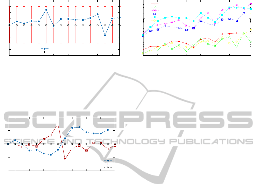
The results show that our system is able to mea-
sure the position of the marker with an accuracy of
about ±1 mm even at a distance of almost 2 meters.
Unfortunately the lasermeter we used only can mea-
sure with an accuracy of ±1.5 mm. Note that the
2
Precaster Enterprises HANS CA770 laser meter. See:
http://www.precaster.com.tw
VISAPP2015-InternationalConferenceonComputerVisionTheoryandApplications
468
-2.5
-2
-1.5
-1
-0.5
0
0.5
1
1.5
2
0 200 400 600 800 1000 1200 1400
Difference [mm]
Relative translation according to the lasermeter [mm]
Optical measurement
Lasermeter
(a) Comparison between the lasermeter and the optical measurement.
0.001
0.01
0.1
1
400 600 800 1000 1200 1400 1600 1800
Standard deviation [mm]/[deg]
Distance to the camera [mm]
t
x
t
y
t
z
R
α
R
β
R
γ
(b) Standard deviations of the measured 6DOF of the marker.
Figure 5: Results of our relative position accuracy measurements from about 400 mm to about 1900 mm distance to the
camera/lasermeter. (a) The plot shows the difference from the optical measurements to the lasermeter. The error bars are due
to the lasermeter. (b) Standard deviations of marker pose parameters in relation to the distance to the camera.
depth accuracy is strongly dependent on the quality
of the intrinsic camera calibration.
-1
-0.5
0
0.5
1
-60 -40 -20 0 20 40 60 80
Difference [deg]
Relative rotation angle according to the goniometer [deg]
Rotation around the x-axis
Rotation around the y-axis
Goniometer
Figure 6: Results of our relative rotation accuracy measure-
ments. The plot shows the difference from the optical mea-
surements to a goniometer.
Next we analyze the rotational accuracy of the
pose estimation. For this, the marker was fixed at a
distance of 1 meter to the camera and attached to a
goniometer. We rotated the marker around its x-axis
from −70
◦
up to 70
◦
and around the y-axis from −60
◦
up to 80
◦
in 10
◦
steps. These angle boundaries are due
to self occlusions of the LED pattern that occur in our
particular experimental setup.
We again recorded 500 measurements at each an-
gle α and compared the relative angle differences. For
this, we converted the marker rotation matrix R
M,α
into the corresponding unit quaternion q
M,α
and cal-
culated the average
¯
q
M,α
. We then determined the
measured relative rotation as the angle of
¯
q
M,α
¯
q
−1
M,0
for every following orientation and compared it to the
goniometer as shown in Figure 6. Our results show
that the rotational measurement error is below ±1
◦
.
4.4 Robustness to Pose Ambiguities
In this experiment we demonstrate the robustness of
the proposed method to pose ambiguities at large dis-
tances to the camera that monocular tracking systems
usually suffer from. For this we fixed the camera on
a static tripod and attached the marker to a wheeled
tripod. Starting at about 50 cm distance to the camera
we recorded a sequence of 2290 frames while manu-
ally moving the marker away up to 7.5 m. Based on
this pre-recorded sequence we monitored the number
of pose flips (Figure 7) using our proposed method
and compared it to the following three other methods:
Method 1: is the simplest approach estimating the
pose by minimizing the reprojection error of only
the six coplanar correspondences i.e.
P
M
= P
1
= argmine
proj
(P,5) (9)
without considering other solutions.
Method 2: also only considers the six coplanar cor-
respondences but makes use of the improvement
of (Schweighofer and Pinz, 2006) by choosing
P
M
= argmin
P∈{P
1
,P
2
}
e
proj
(P,5), (10)
based on the cumulated projection error of all six
correspondences for both solutions.
Method 3: is similar to method 1 but uses all 7 (non-
coplanar) correspondences to determine
P
M
= P
1
= argmine
proj
(P,6), (11)
considering the 3D structure of the marker.
All methods are based on P
H
, the pose roughly esti-
mated from homography.
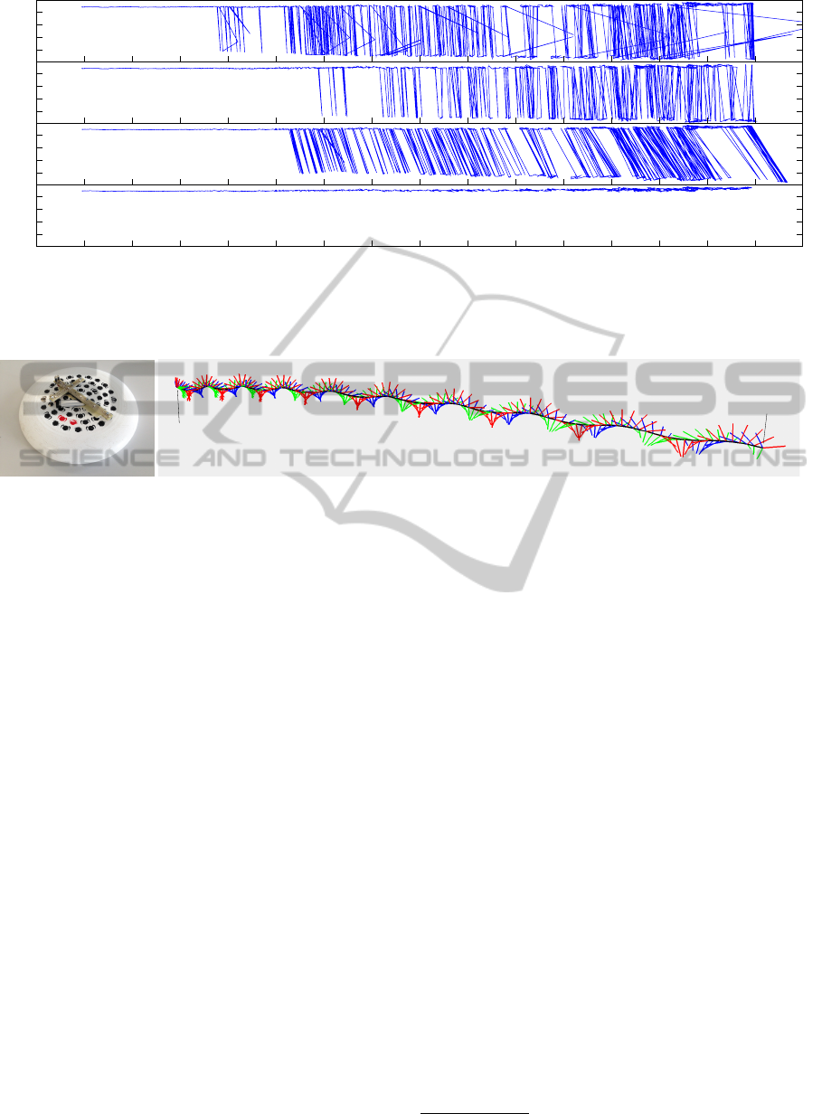
The results show that method 1 performs worst
with the most pose flip occurrences in total, starting
at about 2 meters distance to the camera. Method 2
demonstrates how the strategy of Schweighofer and
Prinz reduces the number of pose flips when using
a purely coplanar marker. Results show that in this
case the flips first occur at a distance of about 3 me-
ters to the camera and that their frequency rises with
increasing distance. Although method 3 performs bet-
ter than method 2 regarding the total number of flips,
High-SpeedandRobustMonocularTracking
469
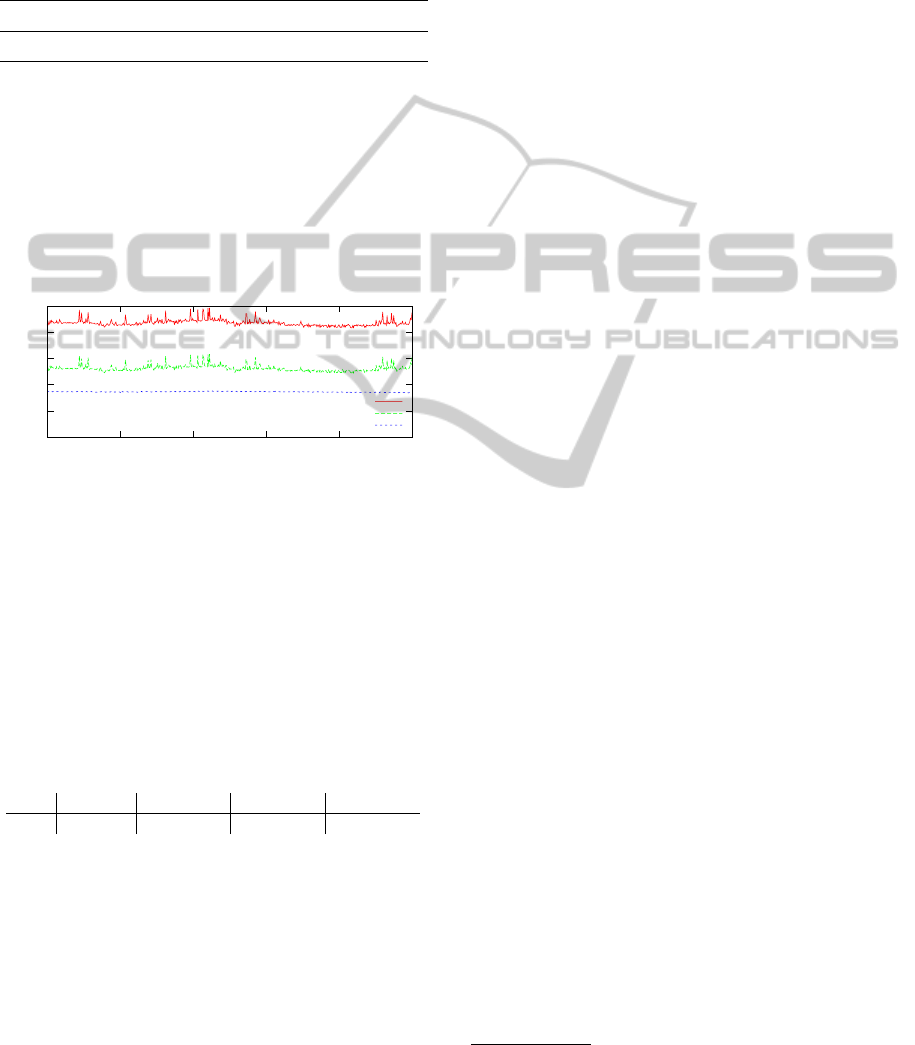
-10
0
10
20
-10
0
10
20
R
α
[deg]
-10
0
10
20
-10
0
10
20
0 500 1000 1500 2000 2500 3000 3500 4000 4500 5000 5500 6000 6500 7000 7500
Distance to the camera [mm]
Method 1: 532 flips
Method 2: 459 flips
Method 3: 426 flips
Proposed: 0 flips
Figure 7: Results of our pose flip comparison experiment. We plot the R
α
in relation to t
z
because it was influenced the most
of all six pose parameters by the flips in our setup. The values are plotted in chronological order from frame 0 to frame 2289.
Negative values of R
α
indicate the occurrence of a pose flip.
(a) Frisbee with the
marker.
t
M,0
t
M,153
(b) A 3D visualization of the tracked trajectory rendered from the cameras perspective.
Figure 8: Results of our rapid motion tracking experiment. (a) The frisbee that was used with the attached prototype marker.
(b) A visualization of the recorded trajectory where we draw the coordinate axes of the marker at each tracked location. The
x-, y- and z-axis of the marker are visualized red, green and blue and their length is equal to the radius of the frisbee (140 mm).
the first flips already occur about 0.5 meters closer to
the camera. It can also be seen that the marker pose
is estimated further away from the camera due to the
elevation of M
6
when the minimization ends up in the
false minimum.
Our proposed method did not flip once in the
whole sequence, which demonstrates the effective-
ness of the pointer LED even at large distances de-
spite its relatively small elevation. In all our exper-
iments we did not manage to cause pose flips in the
range where the LEDs were sufficiently visible to the
camera to determine a pose.
4.5 Robustness to Rapid Motion
In this last experiment we attached the prototype
marker to a frisbee (see Figure 8(a)) in order to
demonstrate the capabilities of our system to robustly
capture rapid motion. The exposure time of the cam-
era was set to 2 ms for this experiment. Although
this hardware setup would not be feasible for a re-
alistic sports analysis of frisbee throws (at least not
in this form), it is still a challenging example of com-
bined rapid translational and rotational movement of a
rigid object. We captured and tracked a 0.955 seconds
long disc throw filmed from diagonal above the scene.
The sequence consists of 154 frames that were all
successfully tracked (see Figure 8(b)). The captured
trajectory
3
started at t
M,0
= (2577.4, 60.3,4564.8)
>
and ended at t
M,153
= (−2896.8,−660.8,7093.4)
>
including nine full turns. Accordingly the frisbee
traveled a total distance of 6.073 meters at an aver-
age speed of approximately 23 km/h. Note that also
in this experiment no pose flips occured.
4.6 Failure Modes
Each marker can only be tracked if all seven LEDs are
visible and separable in the respective frame. Hence
self-occlusions caused by M
6
lead to tracking fail-
ures. Filtering multiple false positive LED detections
fails, if e.g. they appear at different sides around a
marker and therefore do not end up in a single sepa-
rate cluster. When tracking multiple markers, track-
ing will fail if their projected LED patterns are too
close or even overlap due to the nature of the em-
ployed k-means algorithm.
3
All measurements are in mm.
VISAPP2015-InternationalConferenceonComputerVisionTheoryandApplications
470

5 CONCLUSION AND FUTURE
WORK
In this paper, we presented HSRM-Tracking, a
method for robustly estimating and tracking the pose
of multiple infrared markers with a single monocu-
lar camera. Thereby, individual markers can be cor-
rectly recognized in each single camera frame and
distinguished based on the cross ratio of four collinear
LEDs. Our evaluation results show that HSRM-
Tracking is able to precisely capture fine and rapid
movement up to 1000 Hz in a large area neglecting
bandwidth limitations of current cameras.
The proposed method could easily be adapted for
use in a multi-camera system where each camera runs
in parallel in a separate tracking thread. Thus, cam-
eras with different frame rates could be combined to
track the markers asynchronously and contribute to
a synchronized result whenever a new measurement
is available, making camera synchronization unnec-
essary. Being able to estimate the marker pose from a
single camera would also vastly increase the track-
ing volume of a multi camera setup and could be
used in conjunction with stereo methods, whenever
the marker is visible in more than one camera. Such a
setup would also benefit from the LED identification
scheme, since the markers could be used in order to
dynamically calibrate the multi-camera system with-
out having to solve stereo correspondence problems.
REFERENCES
Faessler, M., Mueggler, E., Schwabe, K., and Scaramuzza,
D. (2014). A monocular pose estimation system based
on infrared LEDs. In IEEE International Conference
on Robotics and Automation (ICRA).
Fitzgerald, D., Foody, J., Kelly, D., Ward, T., Markham, C.,
McDonald, J., and Caulfield, B. (2007). Development
of a wearable motion capture suit and virtual reality
biofeedback system for the instruction and analysis of
sports rehabilitation exercises. In EMBS 2007, pages
4870–4874.
Herout, A., Szentandrasi, I., Zacharia, M., Dubska, M., and
Kajan, R. (2013). Five shades of grey for fast and
reliable camera pose estimation. In IEEE Conference
on Computer Vision and Pat. Rec., pages 1384–1390.
Lakemond, R., Fookes, C., and Sridharan, S. (2013).
Resection-intersection bundle adjustment revisited.
ISRN Machine Vision, 2013:8.
Levenberg, K. (1944). A method for the solution of cer-
tain non-linear problems in least squares. Quarterly
Journal of Applied Mathmatics, II(2):164–168.
Lourakis, M. A. and Argyros, A. (2009). SBA: A Software
Package for Generic Sparse Bundle Adjustment. ACM
Trans. Math. Software, 36(1):1–30.
MacKay, D. J. C. (2002). Information Theory, Inference
& Learning Algorithms. Cambridge University Press,
New York, NY, USA.
Marquardt, D. W. (1963). An algorithm for least-squares
estimation of nonlinear parameters. SIAM Journal on
Applied Mathematics, 11(2):431–441.
Naimark, L. and Foxlin, E. (2005). Encoded led system for
optical trackers. In Proceedings of the 4th IEEE/ACM
International Symposium on Mixed and Augmented
Reality, pages 150–153.
Nister, D. (2004). An efficient solution to the five-point
relative pose problem. IEEE Transactions on Pattern
Analysis and Machine Intelligence, 26(6):756–770.
Olson, E. (2011). AprilTag: A robust and flexible vi-
sual fiducial system. In Proceedings of the IEEE In-
ternational Conference on Robotics and Automation
(ICRA), pages 3400–3407. IEEE.
Ong, S. K. and Nee, A. (2004). Virtual Reality and
Augmented Reality Applications in Manufacturing.
Springer Verlag.
Ozuysal, M., Calonder, M., Lepetit, V., and Fua, P. (2010).
Fast keypoint recognition using random ferns. Pat-
tern Analysis and Machine Intelligence, IEEE Trans-
actions on, 32(3):448–461.
Prisacariu, V. and Reid, I. (2012). Pwp3d: Real-time seg-
mentation and tracking of 3d objects. International
Journal of Computer Vision, 98(3):335–354.
Schmaltz, C., Rosenhahn, B., Brox, T., and Weickert, J.
(2012). Region-based pose tracking with occlusions
using 3d models. Machine Vision and Applications,
23(3):557–577.
Schweighofer, G. and Pinz, A. (2006). Robust pose
estimation from a planar target. Pattern Analy-
sis and Machine Intelligence, IEEE Transactions on,
28(12):2024–2030.
Vito, L., Postolache, O., and Rapuano, S. (2014). Mea-
surements and sensors for motion tracking in motor
rehabilitation. Instrumentation Measurement Maga-
zine, IEEE, 17(3):30–38.
Wagner, D., Reitmayr, G., Mulloni, A., Drummond, T., and
Schmalstieg, D. (2008). Pose tracking from natural
features on mobile phones. In Proceedings of the 7th
IEEE/ACM International Symposium on Mixed and
Augmented Reality, pages 125–134.
Welch, G. and Foxlin, E. (2002). Motion tracking: No sil-
ver bullet, but a respectable arsenal. IEEE Comput.
Graph. Appl., 22(6):24–38.
Xu, C., Kuipers, B., and Murarka, A. (2009). 3d pose esti-
mation for planes. In ICCV Workshop on 3D Repre-
sentation for Recognition (3dRR-09).
Yang, H., Wang, F., Xin, J., Zhang, X., and Nishio, Y.
(2012). A robust pose estimation method for nearly
coplanar points. In Proceedings NCSP ’12., pages
345–348.
Zetu, D., Banerjee, P., and Thompson, D. (2000). Extended-
range hybrid tracker and applications to motion and
camera tracking in manufacturing systems. IEEE
Transactions on Robotics and Aut., 16(3):281–293.
High-SpeedandRobustMonocularTracking
471
