
Regularized Latent Least Squares Regression for Unconstrained
Still-to-Video Face Recognition
Haoyu Wang, Changsong Liu and Xiaoqing Ding
State Key Laboratory of Intelligent Technology and Systems
Tsinghua National Laboratory for Information Science and Technology
Department of Electronic Engineering, Tsinghua University, Beijing 100084, China
Keywords:
Still-to-Video Face Recognition, Unconstrained Environment, Regularized Latent Least Squares Regression,
Alternating Optimization.
Abstract:
In this paper, we present a novel method for the still-to-video face recognition problem in unconstrained en-
vironments. Due to variations in head pose, facial expression, lighting condition and image resolution, it is
infeasible to directly matching faces from still images and video frames. We regard samples from these two
distinct sources as multi-modal or heterogeneous data, and use latent identity vectors in a common subspace
to connect two modalities. Differed from the conventional least squares regression problem, unknown latent
variables are treated as response to be computed. Besides, several constraint and regularization terms are in-
troduced into the optimization equation. This method is thus called regularized latent least squares regression.
We divide the original problem into two sub-problems and develop an alternating optimization algorithm to
solve it. Experimental results on two public datasets demonstrate the effectiveness of our method.
1 INTRODUCTION
In recent years, video-based face recognition has
gained more and more traction in both theoretical
and applied research. Though traditional image-based
face recognition has achieved a significant increase
in recognition accuracy, video-based face recognition
is still a challenging problem. Many of existing al-
gorithms can handle faces with moderate variations
in still images, but they are not applicable for video
clips captured in unconstrained environments. Tak-
ing surveillance conditions as an example, a vari-
ety of factors including unknown poses, uncontrolled
lighting and poor video quality may degrade the final
recognition performance. Moreover, due to the diffi-
culty in exploiting useful information and the interfer-
ence from noise, the gain from more video frames is
far less than the increase in time and space complex-
ity.
In this paper, we focus on the still-to-video (S2V)
face recognition problem. While the video-to-video
(V2V) face recognition is to identify faces in query
video sequences against a set of target video se-
quences, the S2V face recognition instead uses still
images as the target set. The S2V face recognition
problem is more practical in real world applications
such as law enforcement, e-passport identification and
video surveillance. In these scenarios, each subject in
gallery set has only one single still image from ID,
passport or driver license. These still images are usu-
ally collected by digital camera in constrained condi-
tion, which are in frontal view, with neutral expres-
sion and normal lighting and of high resolution. In
contrast, video frames in probe set are captured with
ordinary video recorder in unconstrained conditions,
which contain several kinds of variations in pose, fa-
cial expression, illumination and image resolution.
Motion blur and loss of focus introduced during video
capture also result in uncertainty in face representa-
tion.
Based on the fact that still images and video
frames show quite different appearances, it is sensible
to regard these two sources as two different modali-
ties. We assume that face images from the same per-
son in different modalities are identical in some latent
subspace, namely identity space. A face image in one
modality can thus be generated from the identity vec-
tor of this person by a modality-specific transforma-
tion. In reverse, there exists a projection matrix from
each of the two modality spaces into the same iden-
tity space. Regarding the image vector as regressor
and the identity vector as response, we apply regular-
13
Wang H., Liu C. and Ding X..
Regularized Latent Least Squares Regression for Unconstrained Still-to-Video Face Recognition.
DOI: 10.5220/0005267300130020
In Proceedings of the 10th International Conference on Computer Vision Theory and Applications (VISAPP-2015), pages 13-20
ISBN: 978-989-758-090-1
Copyright
c
2015 SCITEPRESS (Science and Technology Publications, Lda.)

ized latent least squares regression with constraints to
find the latent identity vector and projection matrix of
each modality.
To validate the effectiveness of our algorithm, we
conduct experiments on two commonly used video-
based datasets, i.e. COX-S2V (Huang et al., 2012)
and ChokePoint (Wong et al., 2011). Still images and
video frames are used as gallery and probe samples
respectively. We use rank-n average recognition ac-
curacy (rank-n ARA) and cumulative match charac-
teristic (CMC) curve to evaluate the recognition per-
formance. With the help of heterogeneity handling,
our method outperforms most of state-of-the-art algo-
rithms in the S2V face recognition task.
In summary, the major contributions of our work
include three aspects: 1) we regard the S2V face
recognition problem in a way of multi-modal face
recognition; 2) we use regularized latent least squares
regression with constraints method to handle hetero-
geneity; 3) we develop an alternating method to solve
the final optimization problem efficiently.
The rest of the paper is organized as follows: The
next section describes the related work. Section 3 de-
fines the research problem and presents our model and
algorithm. Section 4 evaluates the proposed approach
and confirms its effectiveness. The last section con-
cludes our work and proposes the future work.
2 RELATED WORK
In this section, we briefly introduce several related ap-
proaches dealing with video-based multi-modal face
recognition. In traditional still-to-video (S2V) face
recognition problem, face images from two sources
are regarded as the same. Many classical approaches,
which have achieved considerable performance in
the still-to-still (S2S) face recognition task, are also
applied in the S2V task. The most typical ones
are the well known EigenFace (Turk and Pentland,
1991), FisherFace (Belhumeur et al., 1997) and their
many extensions like (Yang and Liu, 2007), (Tao
et al., 2007), (Tao et al., 2009). Other representative
appearance-based approaches include neighborhood
preserving embedding (NPE) (He et al., 2005a), lo-
cality preserving projections (LPP) (He et al., 2005b)
and their kernelized and tensorized variants. They
can be unified into a general graph embedding (GE)
framework (Yan et al., 2007) under different con-
straints.
However, since the different face appearances of
still images and video frames, such methods prob-
ably fail when simple models cannot handle much
more complex variations in face samples. Several re-
searches have provided specialized algorithms to deal
with such a multi-modal or heterogeneous face recog-
nition problem, where gallery and probe samples are
of distinct modalities. Extended from the descriptions
in (Lei et al., 2012), existing solutions can be catego-
rized by the four stages of a typical face recognition
framework, as shown in Fig. 1.
!"#$%
&'()"*+,"-'.
!$"/0($%
12/("#-'.
30456"#$%
7$"(.+.8
9'+./:3$/%
;"/#<+.8
Figure 1: A typical framework of learning-based multi-
modal face recognition (Lei et al., 2012).
In the stage of face normalization, an intuitive idea
is to synthesize samples by a transformation from
one modality to another, thus matching in the latter
modality. In photo-sketch matching, as one of het-
erogeneous face recognition applications, an eigen-
transformation method (Tang and Wang, 2003) was
firstly proposed to synthesize a sketch from a photo
to match real probe sketch. Local linear embedding
(LLE) (Liu et al., 2005) and Markov random field
(MRF) (Wang and Tang, 2009) were utilized to per-
form the transformation as well. (Wang et al., 2012b)
proposed a semi-coupled dictionary learning method
to simultaneously learn a pair of dictionaries and a
mapping function, which was applied to image super-
resolution and photo-sketch synthesis.
Face features are crucial to the success of face
recognition, so a number of researches focus on fea-
ture descriptors that are invariant to modalities. (Liao
et al., 2009) used difference of Gaussian (DoG) fil-
tering to normalize heterogeneous faces and then ap-
plied multi-block local binary patterns (MB-LBP) to
encode local image structures. (Klare et al., 2011)
improved the recognition accuracy by using scale in-
variant feature transform (SIFT) (Lowe, 1999) and
multi-scale local binary patterns (MLBP) features ex-
tracted from forensic sketches and mug shot photos.
A learning-based couple information-theoreticencod-
ing descriptor was also proposed in (Zhang et al.,
2011) to capture a discriminant local structure in
photo-sketch images.
Subspace learning based methods are another typ-
ical category, which try to find a common subspace
of multi-modal sample spaces to classify heteroge-
neous data. Canonical correlation analysis (CCA)
(Yi et al., 2007), partial least squares (PLS) (Sharma
and Jacobs, 2011) and coupled spectral regression
(CSR) (Lei and Li, 2009) were utilized to formulate a
generic intermediate subspace comparisonframework
for multi-modal recognition. (Kan et al., 2012) pro-
posed the multi-view discriminant analysis (MvDA)
method to jointly solve the multiple linear trans-
VISAPP2015-InternationalConferenceonComputerVisionTheoryandApplications
14

forms by optimizing the between-class and within-
class variations in the common subspace. The partial
and local linear discriminant analysis (PaLo-LDA)
method (Huang et al., 2012) is an LDA’s extension,
taking partial and local constraints into account to dis-
tinguish multi-modal samples.
In order to better measure the similar-
ity/dissimilarity in the video-base face recognition
problem, several point-to-set or set-to-set matching
algorithms are developed other than conventional
statistical methods. Each image set is characterized
as a manifold in manifold-manifold distance (MMD)
model (Wang et al., 2012a) or an affine/convex
hull in AHISD/SHISD model (Cevikalp and Triggs,
2010). (Hu et al., 2012) followed the above work
and proposed the sparse approximated nearest points
(SANP) method, which improved the recognition
performance. The regularized nearest points (RNP)
method (Yang et al., 2013) utilized L2-norm regu-
larization instead of time-consuming L0/L1-norm
sparse constraints and achieved comparable accuracy
as the SANP method.
In this paper, we focus on the subspace learning
stage, leaving the other three stages the same in the
comparison phase.
3 PROPOSED METHOD
In this section, we present our model and algorithm
for the S2V face recognition. We also develop an ef-
ficient algorithm to solve the optimization problem.
3.1 Problem Statement
For the S2V face recognition problem, there are a sin-
gle still image as gallery sample and a set of video
frames as probe samples. The face recognition task is
to match probe samples with the most likely gallery
sample.
More specifically, the problem is formally defined
as follows. Person p has a single still image and n
p
video frames enrolled as sample vectors, which can be
denoted as S
p
= {s
p
} and V
p
= {v
p,1
,v
p,2
,...,v
p,n
p
},
respectively. Let X
S
= {S
1
,S
2
,...,S
P
} and X
V
=
{V
1
,V
2
,...,V
P
} represent sample vectors from two
modalities for all of persons from the training set,
where P is the number of enrolled persons. In the test
phase, assuming V
′
q
= {v
′
q,1
,v
′
q,2
,...,v
′
q,n
′
q
} is a query
video sequence consisting of n
′
q
frames. The label of
V
′
q
is inferred by:
c = argmin
p
d(S
p
,V
′
q
) (1)
where d(S
p
,V
′
q
) is point-to-set distance metric.
3.2 Learning Model
Still images captured by a digital camera have frontal
view, neutral face expression, normal lighting and
high resolution, while video clips captured by a video
recorder have uncertain view, face expression and
lighting, and are usually of low resolution. Many
kinds of variations exist in two modalities, however,
samples of the same identity share much information
in common, which can be regarded as a latent vari-
able. We suppose that samples of the same identity
from two modalities can be generated from an iden-
tical vector in a latent subspace by modality-specific
projections. All the identity vectors are latent vari-
ables in the subspace called identity space, and they
can be classified perfectly from each other. Thus,
through modality-specific projections, sample space
of each modality can be transformed from the iden-
tity space.
3.2.1 Model Formulation
Under the above assumption, both projection matrix
and latent identity vector are unknown variables. As-
suming that the projection from sample space to iden-
tity space is linear transformation, we can formulate
the problem as follows:
y
p
= W
T
S
s
p
+ b
S
(2)
y
p
= W
T
V
v
p,i
+ b
V
, i = 1,2,...,n
p
(3)
where y
p
is the latent identity vector for person p, W
and b are modality-specific projection matrix and bias
term. The subscripts S andV represent two modalities
of still images and video frames. Rewrite Eq. (2) and
(3) in matrix form,
Y
S
= Y = W
T
S
X
S
+ b
S
1
T
N
S
∈ R
m×N
S
(4)
Y
V
= YU = W
T
V
X
V
+ b
V
1
T
N
V
∈ R
m×N
V
(5)
in which
Y = {h
1
,h
2
,...,h
P
} ∈ R
m×P
(6)
U = (u
pq
) ∈ R
P×N
V
, u
pq
=
1, v
N
q
∈ V
p
0, v
N
q
/∈ V
p
(7)
where N
S
= P and N
V
=
∑
P
p=1
n
p
are the total numbers
of still images and video frames, respectively.
As in the multivariate linear regression model, we
use linear least squares approach to estimate unknown
parameters. In Eq. (4) and (5), we treat X as regres-
sor and Y as response. Projection matrices {W}
S,V
and bias terms {b}
S,V
are to be estimated. However,
unlike the classical linear least squares solution, Y
consists of latent identity vectors h
p
for each person,
RegularizedLatentLeastSquaresRegressionforUnconstrainedStill-to-VideoFaceRecognition
15

which cannot be directly used as response. Luck-
ily, under the assumption of identical latent identity
vector, two modalities can be coupled by the identity
space. We utilize this coupling to estimate matrix Y.
The latent least squares regression is formulated as:
min
Y,W,b
{Q
S
(Y,W,b; X) + Q
V
(Y,W,b; X)} (8)
where
Q
S
(Y,W,b; X) =
1
N
S
Y −W
T
S
X
S
− b
S
1
T
N
S
2
F
(9)
Q
V
(Y,W,b; X) =
1
N
V
YU −W
T
V
X
V
− b
S
1
T
N
V
2
F
(10)
and k·k denotes the Frobenius norm of a matrix.
3.2.2 Constraints and Regularizations
Like many other models using least squares approach,
it is necessary to add some constraint and regulariza-
tion terms to prevent overfitting. Due to the limita-
tion of available samples and data sparsity in high-
dimensional space, learning models usually perform
well on training samples but poorly on test samples
from other sources. In our model, we suggest some
heuristics to reduce the search space and computa-
tional complexity. Meanwhile, these constraints also
provide much prior information to improve the gen-
eralization ability of the algorithm. Each of these in-
troduces a optimization term into the original formu-
lation.
Constraint to Preserve Locality. If two faces look
similar in still images, their corresponding identity
vectors would lie close to each other after projections.
This constraint indicates that the projection process
should keep local geometric structures of the still-
image space. Specifically, we describe this assump-
tion in a mathematical form as
G
S
=
N
S
∑
i, j=1
(a
ij
)
S
W
T
S
s
i
−W
T
S
s
j
2
2
(11)
where
(a
ij
)
S
=
(
exp(−
d(s
i
,s
j
)
σ
i
σ
j
), s
i
∈ s
(K)
j
or s
j
∈ s
(K)
i
0, otherwise
(12)
In Eq. (11), G
S
measures the weighed identity-wise
similarity among all identity vectors. The weighing
coefficients are defined as Eq. (12), in which s
(K)
de-
notes the K-nearest neighbors of s, σ is the range of
its K-nearest neighbors and d(s
i
,s
j
) measures the dis-
tance between two samples.
Constraint to Shrink Cluster. Samples of the same
identity in video frames should be clustered together
after projection.
Similar to the idea of LDA (Belhumeur et al., 1997),
this constraint restricts each class by minimizing the
within-class covariance matrix.
G
V
=
N
V
∑
i, j=1
(a
ij
)
V
W
T
V
v
i
−W
T
V
v
j
2
2
(13)
where
(a
ij
)
V
=
(
exp(−
d(v
i
,v
j
)
σ
2
p
), v
i
,v
j
∈ V
p
0, otherwise
(14)
(a
ij
)
V
takes cluster scale into account and uses rela-
tive distance instead of constants to control weighting
coefficients. σ
p
denotes the maximum of d(v
i
,v
j
) for
∀v
i
,v
j
∈ V
p
.
Regularization to Penalize Complexity. Extreme
parameter values should be prevented in projection
matrices.
We apply the commonly used regularization method
as kWk
2
F
to restrict coefficients in two matrices.
In summary, Eq. (11) and (13) can be rewritten in
matrix form.
G
S
(W; X) = trace((W
T
S
X
S
)L
S
(W
T
S
X
S
)
T
) (15)
G
V
(W; X) = trace((W
T
V
X
V
)L
V
(W
T
V
X
V
)
T
) (16)
where L = D − A is the Laplacian matrix and D is a
diagonal matrix with d
ii
=
∑
j
a
ij
. And we define the
regularization term as
R(W) = kW
S
k
2
F
+ kW
V
k
2
F
(17)
3.2.3 Final Model and Solution
By combining the above three constraint and regular-
ization terms with the original formulation Eq. (8),
the optimization problem is finally obtained as
min
Y,W,b
{Q
S
(Y,W,b; X) + Q
V
(Y,W,b; X)
+α
S
G
S
(W; X) + α
V
G
V
(W; X) + βR(W)}
s.t. kY
p
k
2
2
= 1, p = 1,2,...,P
(18)
where terms are sequentially defined in Eq. (9) (10)
(15) (16) (17). α
S
, α
V
, β are balance parameters. Y
p
denotes the pth column vector of matrix Y, which is
normalized to unit length.
In order to solve Eq. (18), we use an alternat-
ing minimization method, which is efficient to solve
multiple variable optimization problems. The origi-
nal problem is divided into two sub-problems, where
{Y} and {W,b}
S,V
are optimized alternatingly with
VISAPP2015-InternationalConferenceonComputerVisionTheoryandApplications
16

the other group fixed. The two sub-problems are de-
fined as follows.
Sub-problem 1. Given H, find {W, b}.
min
W,b
J
1
(W,b; X,Y)
= Q
S
(W,b; X,Y) + Q
S
(W,b; X,Y)
+ α
S
G
S
(W; X) + α
V
G
V
(W; X) + βR(W)
(19)
Sub-problem 2. Given {W, b}, find Y.
min
Y
J
2
(Y; X,W,b)
= Q
S
(Y; X,W,b) + Q
V
(Y; X,W,b)
s.t. kY
p
k
2
2
= 1, p = 1,2,...,P
(20)
Sub-problem 1 has no analytical solutions so that we
instead use gradient descent (GD) method to solve it.
Sub-problem 2 has an analytical solution and we cal-
culate the optimized Y directly. For more details of
solution process, please refer to Appendix.
In summary, Algorithm 1 shows the procedure of
optimization algorithm as described above.
Algorithm 1: Regularized Latent Least Squares Re-
gression with Constraints
Input: The training sets X
S
∈ R
m×N
S
and X
V
∈
R
m×N
V
, balance parameters {α,β}, maximum it-
eration number T.
Output: The identity vectors Y, projection matrices
{W}
S,V
, bias terms {b}
S,V
.
1: Initialize Y randomly and normalize kY
p
k
2
2
= 1,
Y
p
is Y’s column vector.
2: Set iter = 0.
3: while not converged and iter < T do
4: Update W,b by solving Eq. (19), with Y fixed;
5: Update Y by solving Eq. (20), with W,b fixed;
6: Normalize kY
p
k
2
2
= 1;
7: Set iter = iter + 1;
8: end while
9: return Y,{W}
S,V
,{b}
S,V
4 EXPERIMENTS
In this section, we incorporate our proposed method
in the whole S2V face recognition framework. We
discuss the experimental setting and evaluate the al-
gorithm on two public datasets.
4.1 Experimental Setting
Two video-based face recognition datasets, COX-
S2V (Huang et al., 2012) and ChokePoint (Wong
et al., 2011), are used to evaluate our method. Im-
age samples for training and test, which are available
in both datasets, are faces detected and cropped from
original video clips. To allow comparison with the lit-
erature, only histogram equalization is performed and
no other preprocessing is included. Face images are
resized to 96 × 120 in COX-S2V dataset and 96× 96
in ChokePoint dataset. Raw gray-scale pixel values
are concatenated to form feature vectors. Feature vec-
tors from each modality are first processed by PCA
and 98 percent of energy is preserved.
The conventional training-validation-test scheme
is applied in the framework. In the training phase,
still images and video frames are enrolled as X
S
and
X
V
, thus projection matrix for each modality can be
learnt by the model described in Section 3. A 5-fold
cross validation is performed during this phase to find
the most suitable values of parameters {m,α
S
,α
V
,β}.
In our experiments, m = 120, α
S
= 0.05, α
V
= 0.01,
β = 0.05 are set for COX-S2V dataset, and m = 90,
α
S
= 0.1, α
V
= 0.02, β = 0.02 are set for Choke-
Point dataset. In the test phase, still images are en-
rolled as the gallery set and video sequences as the
probe set. By projecting probe video frames into the
identity space, similarity scores between the probe
and each gallery sample are obtained. If the top-n
similar gallery samples contain the exact probe iden-
tity, recognition of this probe is recorded as correct
in rank-n recognition accuracy measure. The cumula-
tive match characteristic (CMC) curve illustrates the
cumulative accuracy rate with respect to rank-n.
The proposed method is compared with several
existing methods for the S2V face recognition prob-
lem. Subspace learning based and discriminant anal-
ysis based methods are included for comparison, e.g.
LDA (Belhumeur et al., 1997), CCA (Yi et al., 2007),
PLS (Sharma and Jacobs, 2011), CSR (Lei and Li,
2009), MvDA (Kan et al., 2012) and PaLo-LDA
(Huang et al., 2012). Above algorithms are imple-
mented either by using source codes provided by the
authors or by ourselves according to the literature, all
with model parameters tuned.
4.2 Experimental Results and Analysis
4.2.1 COX-S2V Dataset
The COX-S2V dataset contains 1,000 persons, with
each person a controlled still image and four uncon-
trolled video clips, each consisting of approximately
25 frames. The still images are captured by a high
quality digital camera. The four video sequences are
collected by two different off-the-shelf camcorders at
two different distances away from the subjects. While
RegularizedLatentLeastSquaresRegressionforUnconstrainedStill-to-VideoFaceRecognition
17
video recording, subjects walk naturally without any
restrictions on head pose or face expression. Such
a setting provides a good simulation of real video
surveillance scenarios in term of lighting condition
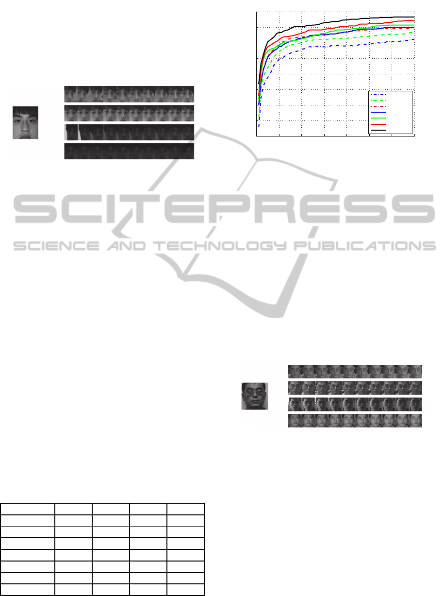
and image resolution. Some examples are shown in
Fig. 2.
Figure 2: A still image and some frames of four video se-
quences of a subject from the COX-S2V dataset.
According to the protocol, the whole dataset is di-
vided into non-overlapping 300 and 700 persons for
training and test, respectively. The results are sum-
marized in Table 1. Since video3&4 are captured
in a backlight environment, image quality is poorer
than that of video1&2, thus the recognition accuracy
is significantly lower. Besides, due to the relatively
near distance from subjects, the results of video2&4
are better than those of video1&3, which indicates
the effect of image resolution. In general, our pro-
posed method outperforms all other methods in all
of the four subsets. It shows much more robustness
in head pose, illumination, resolution and other im-
age variations, which proves the effectiveness of our
model. Contrary to our expectation, classical LDA,
i.e. FisherFace, has better performance than many of
algorithms that are designed to handle heterogeneity.
This may be explained by the advantage in general-
ization ability of naive models over complex models.
More specifically, the CMC curve on subset video2 is
drawn in Fig. 3. It shows that our method achieves su-
periority all along the top-10% (70 out of 700) ranks.
Over 98% of correctly recognized identities can be
found in the top-10% returned results.
Table 1: Rank-1 recognition accuracy (%) on four subsets
of COX-S2V dataset.
Method video1 video2 video3 video4
LDA 48.86 71.86 20.71 55.86
CCA 45.00 62.29 18.43 52.57
PLS 47.71 65.57 18.86 52.43
CSR 50.86 69.29 23.14 52.71
MvDA 50.71 70.14 21.14 55.43
PaLo-LDA 52.43 73.00 22.00 56.71
Proposed 54.28 76.71 24.14 58.57
0 10 20 30 40 50 60 70
0.6
0.65
0.7
0.75
0.8
0.85
0.9
0.95
1
Rank
Cumulative Recognition Rate
CCA
PLS
CSR
MvDA
LDA
PaLo−LDA
Proposed
Figure 3: CMC curve on subset video2 of COX-S2V
dataset.
4.2.2 ChokePoint Dataset
The ChokePoint dataset is designed for experiments
in person identification/verification under real-world
surveillance conditions. In total, it consists of 48
video sequences and 64,204 face images. Sequences
are recorded on two distinct portals, with entering and
leaving modes for each portal. In each type of portal
setting, three cameras placed above a door simulta-
neously record from three viewpoints, and four se-
quences are recorded repeatedly to enroll variations.
Though walking directions may vary, the setting of
three viewpoints allow for the capture of near-frontal
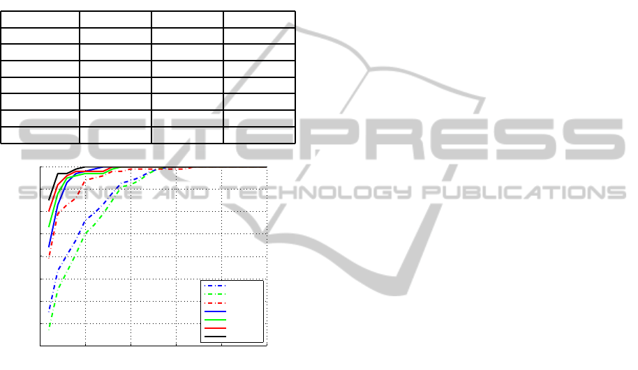
faces. Some examples are shown in Fig. 4.
Figure 4: A still image and some frames of selected video
sequences of a subject from the ChokePoint dataset.
According to the provided protocol, 16 out of 48
video sequences should be selected and divided into
two groups for development and evaluation. How-
ever, differed from the video-to-video verification
task, our still-to-video identification task uses the only
one still image and 16 selected video sequences for
each of the 25 subjects. Therefore, 8 out of the 16
video sequences are randomly selected for training
and the remaining half for test. The experiment is
formulated as a close-set identification problem and
evaluated with a 10-fold validation scheme. The re-
sults are summarized in Table 2. We also conduct ex-
periments on various numbers of frames to test their
VISAPP2015-InternationalConferenceonComputerVisionTheoryandApplications
18
robustness in probe set size. Our proposed method
can achieve better performance than other methods,
and merely drops a little as the decrease in frame
number. Fig. 5 illustrates the CMC curve of seven
methods used for comparison, with 50 frames in each
probe video sequence. Our proposed method, as the
black line shows, has the highest recognition rate and
reaches 100% accuracy after rank = 5.
Table 2: Average rank-1 recognition accuracy (%) on
ChokePoint dataset.
Method 10 frames 30 frames 50 frames
LDA 74.25 81.40 86.45
CCA 51.35 61.00 67.50
PLS 50.75 56.90 63.55
CSR 61.15 74.40 79.40
MvDA 75.40 78.95 81.95
PaLo-LDA 82.35 87.40 90.05
Proposed 87.90 91.30 92.50
0 5 10 15 20 25
0.6
0.65
0.7
0.75
0.8
0.85
0.9
0.95
1
Rank
Cumulative Recognition Rate
CCA
PLS
CSR
MvDA
LDA
PaLo−LDA
Proposed
Figure 5: CMC curve on ChokePoint dataset with 50 frames
in each video sequence.
5 CONCLUSIONS
This paper proposes an effective regularized least
squares regression with constraints for unconstrained
still-to-video face recognition. The S2V face recogni-
tion is treated as a multi-modal or heterogeneous face
recognition problem. Latent identity subspace is en-
rolled as the linkage between two modalities. In addi-
tion to the conventional least squares regression, con-
straint and regularization terms are introduced into
the optimization equation to enhance generalization
ability and reduce computational complexity. An al-
ternating optimization algorithm is developed on the
basis of two sub-problems. Experimental results on
two public datasets demonstrate that our method can
perform significantly better than many relevant algo-
rithms in the literature.
For future work, we will focus on how to handle
larger variations in head pose. Splitting a continuous
video sequence into several subsets after pose estima-
tion is a possible solution. Besides, based on exist-
ing set-to-set matching algorithms, how to effectively
measure similarity/dissimilarity between a point and
a point set is also an interesting topic.
ACKNOWLEDGEMENTS
This work was supported by the National Basic Re-
search Program of China (973 program) under Grant
No. 2013CB329403.
REFERENCES
Belhumeur, P. N., Hespanha, J.P., and Kriegman, D. (1997).
Eigenfaces vs. Fisherfaces: Recognition using class
specific linear projection. IEEE Trans. Pattern Analy-
sis and Machine Intelligence, 19(7):711–720.
Cevikalp, H. and Triggs, B. (2010). Face recognition based
on image sets. In Proc. IEEE Conference on Com-
puter Vision and Pattern Recognition, pages 2567–
2573. IEEE.
He, X., Cai, D., Yan, S., and Zhang, H.-J. (2005a). Neigh-
borhood preserving embedding. In Proc. 10th IEEE
International Conference on Computer Vision, vol-
ume 2, pages 1208–1213. IEEE.
He, X., Yan, S., Hu, Y., Niyogi, P., and Zhang, H.-
J. (2005b). Face recognition using Laplacianfaces.
IEEE Trans. Pattern Analysis and Machine Intelli-
gence, 27(3):328–340.
Hu, Y., Mian, A. S., and Owens, R. (2012). Facerecognition
using sparse approximated nearest points between im-
age sets. IEEE Trans. Pattern Analysis and Machine
Intelligence, 34(10):1992–2004.
Huang, Z., Shan, S., Zhang, H., Lao, S., Kuerban, A., and
Chen, X. (2012). Benchmarking still-to-video face
recognition via partial and local linear discriminant
analysis on COX-S2V dataset. In Proc. 11th Asian
Conference on Computer Vision, Volume Part II, pages
589–600. Springer-Verlag.
Kan, M., Shan, S., Zhang, H., Lao, S., and Chen, X. (2012).
Multi-view discriminant analysis. In Proc. 12th Euro-
pean Conference on Computer Vision, Volume Part I,
pages 808–821. Springer-Verlag.
Klare, B. F., Li, Z., and Jain, A. K. (2011). Matching foren-
sic sketches to mug shot photos. IEEE Trans. Pattern
Analysis and Machine Intelligence, 33(3):639–646.
Lei, Z. and Li, S. Z. (2009). Coupled spectral regression for
matching heterogeneous faces. In Proc. IEEE Con-
ference on Computer Vision and Pattern Recognition,
pages 1123–1128. IEEE.
Lei, Z., Liao, S., Jain, A. K., and Li, S. Z. (2012). Coupled
discriminant analysis for heterogeneous face recogni-
RegularizedLatentLeastSquaresRegressionforUnconstrainedStill-to-VideoFaceRecognition
19

tion. IEEE Trans. Information Forensics and Security,
7(6):1707–1716.
Liao, S., Yi, D., Lei, Z., Qin, R., and Li, S. (2009). Het-
erogeneous face recognition from local structures of
normalized appearance. In Proc. International Con-
ference on Advances in Biometrics, pages 209–218.
Springer-Verlag.
Liu, Q., Tang, X., Jin, H., Lu, H., and Ma, S. (2005). A non-
linear approach for face sketch synthesis and recogni-
tion. In Proc. IEEE Computer Society Conference on
Computer Vision and Pattern Recognition, volume 1,
pages 1005–1010. IEEE.
Lowe, D. G. (1999). Object recognition from local scale-
invariant features. In Proc. IEEE International Con-
ference on Computer Vision, volume 2, pages 1150–
1157. IEEE.
Sharma, A. and Jacobs, D. W. (2011). Bypassing synthesis:
PLS for face recognition with pose, low-resolution
and sketch. In Proc. IEEE Conference on Com-
puter Vision and Pattern Recognition, pages 593–600.
IEEE.
Tang, X. and Wang, X. (2003). Face sketch synthesis and
recognition. In Proc. 9th IEEE International Confer-
ence on Computer Vision, pages 687–694. IEEE.
Tao, D., Li, X., Wu, X., and Maybank, S. J. (2007). Gen-
eral tensor discriminant analysis and gabor features
for gait recognition. IEEE Trans. Pattern Analysis and
Machine Intelligence, 29(10):1700–1715.
Tao, D., Li, X., Wu, X., and Maybank, S. J. (2009). Geo-
metric mean for subspace selection. IEEE Trans. Pat-
tern Analysis and Machine Intelligence, 31(2):260–
274.
Turk, M. A. and Pentland, A. P. (1991). Face recognition
using Eigenfaces. In Proc. IEEE Computer Society
Conference on Computer Vision and Pattern Recogni-
tion, pages 586–591. IEEE.
Wang, R., Shan, S., Chen, X., Dai, Q., and Gao, W.
(2012a). Manifold–manifold distance and its applica-
tion to face recognition with image sets. IEEE Trans.
Image Processing, 21(10):4466–4479.
Wang, S., Zhang, D., Liang, Y., and Pan, Q. (2012b). Semi-
coupled dictionary learning with applications to im-
age super-resolution and photo-sketch synthesis. In
Proc. IEEE Conference on Computer Vision and Pat-
tern Recognition, pages 2216–2223. IEEE.
Wang, X. and Tang, X. (2009). Face photo-sketch synthesis
and recognition. IEEE Trans. Pattern Analysis and
Machine Intelligence, 31(11):1955–1967.
Wong, Y., Chen, S., Mau, S., Sanderson, C., and Lovell,
B. C. (2011). Patch-based probabilistic image qual-
ity assessment for face selection and improved video-
based face recognition. In Proc. IEEE Computer
Society Conference on Computer Vision and Pattern
Recognition Workshops, pages 74–81. IEEE.
Yan, S., Xu, D., Zhang, B., Zhang, H.-J., Yang, Q., and Lin,
S. (2007). Graph embedding and extensions: a general
framework for dimensionality reduction. IEEE Trans.
Pattern Analysis and Machine Intelligence, 29(1):40–
51.
Yang, J. and Liu, C. (2007). Horizontal and vertical
2DPCA-based discriminant analysis for face verifica-
tion on a large-scale database. IEEE Trans. Informa-
tion Forensics and Security, 2(4):781–792.
Yang, M., Zhu, P., Van Gool, L., and Zhang, L. (2013).
Face recognition based on regularized nearest points
between image sets. In Proc. 10th IEEE International
Conference and Workshops on Automatic Face and
Gesture Recognition, pages 1–7. IEEE.
Yi, D., Liu, R., Chu, R., Lei, Z., and Li, S. Z. (2007). Face
matching between near infrared and visible light im-
ages. In Proc. International Conference on Advances
in Biometrics, pages 523–530. Springer-Verlag.
Zhang, W., Wang, X., and Tang, X. (2011). Coupled
information-theoretic encoding for face photo-sketch
recognition. In Proc. IEEE Conference on Com-
puter Vision and Pattern Recognition, pages 513–520.
IEEE.
APPENDIX
This appendix demonstrates the solution of two sub-
problems defined in Section 3.
As in Eq. (19), Y is given and {W, b} is to be ob-
tained by minimizing J
1
(W,b; X,Y). Since there are
no analytical solutions, we use the gradient descent
(GD) method to minimize the expression. We com-
pute the derivatives of J
1
with respect to W and b as
(taking W
S
and b
S
as example):
∂J
1
∂W
S
= −
2
N
S
X
S
(Y −W
T
S
X
S
− b
S
1
T
N
S
)
T
+ 2α
S
W
T
S
X
S
L
S
X
T
S
+ 2βW
T
S
∂J
1
∂b
S
= −
2
N
S
(Y −W
T
S
X
S
− b
S
1
T
N
S
)1
N
S
Thus, the matrices can be updated by the above
gradients until convergence.
W
S
= W
S
− γ
∂J
1
∂W
S
, b
S
= b
S
− γ
∂J
1
∂b
S
As in Eq. (20), {W,b} is given and Y is to be
obtained by minimizing J
2
(Y; X,W, b). Consider the
derivative of J
2
with respect to Y
∂J
2
∂Y
=
2
N
S
(Y −W
T
S
X
S
− b
S
1
T
N
S
)
+
2
N
V
(YU − W
T
V
X
V
− b
V
1
T
N
V
)U
T
Let it be zero and obtain
Y =
1
N
S
(W
T
S
X
S
+ b
S
1
T
N
S
) +
1
N
V
(W
T
V
X
V
+ b
V
1
T
N
V
)U
T
×
1
N
S
I +
1
N
V
UU
T
−1
VISAPP2015-InternationalConferenceonComputerVisionTheoryandApplications
20
