
Spectral Fiber Feature Space Evaluation for Crime Scene Forensics
Traditional Feature Classification vs. BioHash Optimization
Christian Arndt
1
, Jana Dittmann
1,2
and Claus Vielhauer
1,3
1
Otto-von-Guericke University Magdeburg, Dept. of Computer Science, Research Group Multimedia and Security,
PO box 4120, 39016 Magdeburg, Germany
2
University of Buckingham, Applied Computing Dept., Buckingham MK18 1EG, U.K.
3
Brandenburg University of Applied Sciences, Informatics and Media Dept., PO box 2132, 14737 Brandenburg, Germany
Keywords:
Digitized Crime Scene Forensics, Fiber Analysis, Identification, Individualization, Feature Space Evaluation.
Abstract:
Despite of ongoing improvements in the field of digitized crime scene forensics, a lot of analysis work is
still done manually by trained experts. In this paper, we derive and define a 2048 dimensional fiber feature
space from a spectral scan with a wavelength range of 163 - 844 nm sampled with FRT thin film reflectometer
(FTR). Furthermore, we perform an evaluation of seven commonly used classifiers (Naive Bayes, SMO, IBk,
Bagging, Rotation Forest, JRip, J48) in combination with a proven concept from the biometric field of user
authentication called Biometric Hash algorithm (BioHash). We perform our evaluation in two well-known
forensic examination goals: identification - determining the broad fiber group (e.g. acrylic) and individual-
ization - finding the concrete textile originator. Our experimental test set considers 50 different fibers, each
sampled in four scan resolutions of: 100, 50, 20, 10 µm. Overall, 800 digital samples are measured. For
both examination goals we can show that despite the Naive Bayes all classifiers show a positive classification
tendency (80 - 99%), whereby the BioHash optimization performs best for individualization tasks.
1 INTRODUCTION
Alongside classic biometric traits such as fingerprints
and face other trace types also play an important role
in forensic crime scene investigations, such as textile
fiber traces as a subcategory of micro traces. Nowa-
days, in the field of forensic fiber analysis, a trained
expert’s work is time-consuming and cost-intensive.
Analysis work is often performed manually with only
limited computing science support (SWGMAT, 1999;
Houck and Siegel, 2010). Subjective expert’s obser-
vations/decisions can be supported/strengthened by
non-destructive and reproducible machine estimation.
Fibers indwell a high evidential value for various
reasons. Besides their appearance in numerous high-
profile cases, they rank among the frequently encoun-
tered physical evidence (Houck and Siegel, 2010).
Since textiles and clothes are ubiquitous, fibers can
potentially occur everywhere, even on crime scenes.
One fundamental rule therefore is Locard’s exchange
principle - “Every contact leaves a trace”. This
quote states that no one can act/commit a crime with
force/intensity without leaving numerous signs/marks
(Inman and Rudin, 2001).
Apart from typical physical fiber characteristics - like
diameter, delustrant, (reduces the sheen of chemical
fibers), cross-sectional shape and morphological sur-
face structure - fiber color also plays an important
role. Although fiber color is one of the most distin-
guishing fiber characteristics (SWGMAT, 1999), it is
also one of the most underutilized traits (Houck and
Siegel, 2010). Hence, color should be analyzed spec-
trally and/or chemically. Therefore, we use a FRT
thin film reflectometer (FTR) in our feature evalua-
tion approach to cover both requirements. In respect
to prior work, for a contactless and non-destructive
data acquisition a chromatic white light sensor (CWL)
(Hildebrandt et al., 2012) and a confocal laser scan-
ning microscope (CLSM) (Arndt et al., 2012) were
already evaluated regarding their technical suitabil-
ity. Besides new opportunities in optical and spectral
sensing, computing science offer several signal and
pattern recognition techniques to support experts and
derive result indications. Prior work has shown a pos-
itive result tendency regarding a computer-aided fiber
identification - determining the broad fiber category
- using supervised learning (Hildebrandt et al., 2012)
as well as template matching (Arndt et al., 2012).
293
Arndt C., Dittmann J. and Vielhauer C..
Spectral Fiber Feature Space Evaluation for Crime Scene Forensics - Traditional Feature Classification vs. BioHash Optimization.
DOI: 10.5220/0005270402930302
In Proceedings of the 10th International Conference on Computer Vision Theory and Applications (VISAPP-2015), pages 293-302
ISBN: 978-989-758-089-5
Copyright
c
2015 SCITEPRESS (Science and Technology Publications, Lda.)

Therefore, we consider both matching methodolo-
gies in our experiments. Seven different supervised
classifiers in a 2048 dimensional feature space and
a template matching approach derived from the Bio-
metric Hash algorithm (BioHash), introduced in bio-
metrics (Vielhauer, 2006), are evaluated. By apply-
ing the known BioHash algorithm from the biometric
field of dynamic handwriting, we want to compen-
sate the intra-class variability of our spectral measure-
ment data. Finally, we want to evaluate typical classi-
fiers regarding their performance and the optimization
impact of the BioHash algorithm within the feature
space of 2048 spectral features from FTR sensing. We
prepare, measure and evaluate 50 different fibers in
four acquisition resolutions of: 100, 50, 20, 10 µm in
our experiments. In summary, 400 scan samples are
used for training and classification. Based on forensic
case work, we consider two test goals: identification
- determining the broad fiber category out of 5 differ-
ent groups (e.g. acrylic) and individualization - find-
ing the concrete textile originator out of 25 specific
fiber types. In summary, we pursue three test objec-
tives: O1 for identification, O2 for individualization
and O3 for comparing both aforementioned objectives
by their achieved results.
This paper is structured as follows: In 2 we sum-
marize the relevant state of the art and related work.
The conceptual basis of our approach is introduced
in 3. A detailed description of our experimental test
setup is given in 4. Hereafter, obtained results are pre-
sented. Finally, we summarize our findings and derive
future tasks in 6.
2 STATE OF THE ART
This section gives an overview of related research
work in the field of forensic fiber analysis, relevant
biometric topics and the used sensing device.
2.1 Forensic Fiber Analysis
Houck and Siegel define a textile fiber as a “unit
of matter, either natural or manufactured, that forms
the basic element of fabrics and other textiles [...]”.
This definition also describes the two main fiber cat-
egories: natural - a fiber, which exists in a natural
state (e.g. plant fiber - cotton or animal hair - wool),
chemical - derived from any substance by a process of
manufacture (e.g. synthetic polymer - acrylic) (Houck
and Siegel, 2010). Common forensic trace work starts
with the physical trace acquisition on a crime scene.
Every process step hereafter is done under labora-
tory conditions. Nowadays, textile fibers are typically
analyzed in a manual manor by trained experts with
the help of special microscopes (SWGMAT, 1999).
Achieved results are based on subjective expert deci-
sions and often hard to comprehend and reproduce.
In a first examination step called identification
(one-to-many comparison), a fiber trace is tentatively
assigned to a broad group (e.g. natural or chemical
fibers) based on characteristic optical features (e.g.
surface characteristics), in order to limit the number
of potential garments for individualization. Individu-
alization on the contrary is perceived as the ultimate
goal in forensic examination and it is denoted by a
one-to-one comparison, searching for the textile ori-
gin (Inman and Rudin, 2001).
2.2 Related Work
Different spectrography-based research approaches in
the context of textile fiber identification and individu-
alization were already presented. Standard test meth-
ods encourage the usage of absorption spectra to dis-
tinguish between chemical fibers (AST, 2000). Sto-
effler et al. (Stoeffler, 1996) introduced a flowchart
system for the identification (nine generic classes) of
synthetic fibers by transmissive polarized light mi-
croscopy. Another nondestructive approach presented
by Prange et al. (Prange et al., 1995) based on total re-
fection x-ray fluorescence (TXRF) uses characteristic
trace element pattern for fiber identification. With the
help of these “fiber fingerprints” 23 out of 35 samples
(test-set contains: polyester, wool and viscose) were
correctly assigned. Another differentiation technique
using terahertz (THz) transmittance spectroscopy is
introduced by Kurabayashi et al. (Kurabayashi et al.,
2010). A three-dimensional excitation-emission ma-
trix as feature space is utilized by Appalaneni et al.
for the comparison of single fiber dyes (Appalaneni
et al., 2014). Millington (Millington, 2012) uses UV-
visible diffuse reflectance spectroscopy to analyze the
color of undyed fibrous materials in the CIE XYZ
color space. Nowadays Fourier transform infrared
spectroscopy (FTIR) is the preferred method to de-
termine fiber material properties (Houck and Siegel,
2010).
The FRT FTR thin film reflectometer (Fries Re-
search & Technology GmbH (FRT), 2010) was al-
ready evaluated regarding the visibility assessment
of latent fingerprints on challenging surfaces (Hilde-
brandt et al., 2013). This briefly summarized re-
lated work shows that several fiber identification ap-
proaches were successfully using either transmis-
sive or reflectance spectrography-based sensing tech-
niques.
A lot of research has been done so far in the field
VISAPP2015-InternationalConferenceonComputerVisionTheoryandApplications
294
of fiber identification, whereas the individualization
gets only scarce attention. The German state police
in Saxony-Anhalt and Berlin measure also the fiber
absorption by transmittance-based FTIR techniques
(UV-VIS wavelength range) for the purpose of fiber
individualization.
2.3 Biometric Hash Algorithm
First test scans showed fluctuations within the fiber
reflectance spectra of the same sample, similar to nat-
ural variations of biometric traits. The observation
leads to the assumption that our feature space needs
to be optimized regarding the intra-class variability of
a sample, whilst preserving its discriminatory power.
This is where the following algorithm comes into
play.
The Biometric Hash algorithm (hereafter Bio-
Hash), introduced by Vielhauer et al. (Vielhauer et al.,
2002), is intentionally designed for online authenti-
cation in the field of dynamic biometric handwriting
recognition. It is based on the idea of extracting a spe-
cific number of statistical features from a biometric
raw signal that possesses a high intra-class variabil-
ity. As a result of the BioHash generation the features
are projected into a more stable representation, which
minimizes the intra-class variability (fluctuations of
feature manifestations of the same originator). The
approach considers a transformation of every newly
acquired biometric data sample into the BioHash fea-
ture space representation by means of special helper
data. This helper data is called Interval Matrix IM,
consisting of two vectors containing mapping interval
lengths and offsets for each feature. During an enroll-
ment process (training phase of a biometric system) to
compensate the natural variability of handwriting, this
particular IM generation is performed. Moreover, it is
necessary to parameterize the BioHash generation by
scaling the mapping intervals with the help of: Tol-
erance Vector TV - local impact of intra-class, indi-
vidual feature variability and global Tolerance Factor
TF - controls the tolerance of feature variability above
the entire feature set. A more detailed description is
given in (Vielhauer, 2006).
3 CONCEPT
In this section we propose our concept to address the
identified research challenge.
Basically, our idea is to combine spectral measure-
ment results of the FTR sensor with the Biometric
Hash algorithm as matching methodology in order to
minimize the intra-class variability. Our overall aim is
to classify textile fibers correctly based on their digi-
tal measurement data in both forensic use case scenar-
ios - identification and individualization (see follow-
ing 3.1 for pursued objectives). Besides this, the FTR
sensor is evaluated regarding the suitability for digi-
tal fiber data acquisition. The discriminatory power
of acquired spectral fiber measurement data is inves-
tigated as well.
To evaluate the FTR sampled 2048 dimensional
feature space consisting of raw spectral data, as well
as BioHash results, we suggest to use common pattern
recognition pipelines as known e.g. from Jain (Jain,
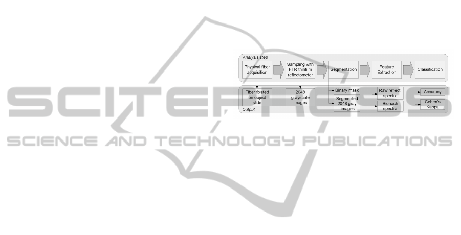
1989), Vielhauer (Vielhauer, 2006) (see 1).
Figure 1: Fiber analysis pipeline for spectral classification.
3.1 Pursued Objectives
We derive our addressed objectives in relation to the
well-known forensic uses cases (see 2).
O1 - Identification Assign the currently analyzed
fiber to the correct broad category based on:
O1.1 - raw, unaltered spectral data
O1.2 - BioHash spectral data
O2 - Individualization Assign the currently ana-
lyzed fiber to the correct textile origin based on:
O2.1 - raw, unaltered spectral data
O2.2 - BioHash spectral data
O3 - Classification evaluation Compare both fea-
ture spaces by calculating the difference between
raw and BioHash classifier performance:
O3.1 - for O1 identification
O3.2 - for O2 individualization
As quality measures for objective O1 and O2 the clas-
sifier prediction performance is evaluated using accu-
racy and Cohen’s Kappa coefficient. Accuracy (cor-
rect classification rate in percent) is calculated by the
number of correct assignments divided by the total of
the population (0% - only false assignments, 100% -
only correct assignments). The agreement between
predicted and observed categorizations is measured
by Kappa statistics (1 - 100% complete agreement,
0 - guess, negative values - beyond guessing) (Hall
et al., 2009). The potential BioHash performance
SpectralFiberFeatureSpaceEvaluationforCrimeSceneForensics-TraditionalFeatureClassificationvs.BioHash
Optimization
295

boost is measured for O3 by calculating the differ-
ence between BioHash and raw classification results
in percent.
3.2 Proposed Analysis Pipeline
All utilized physical specimen are extracted either
from labelled used clothes or new fiber threads with
information about the origin. Different colors are cho-
sen on purpose to consider this important characteris-
tic. The test set, consisting of new and worn fibers,
should clarify the question about the individualiza-
tion ability - Can new fibers without individualiza-
tion characteristics be individualized as well? Con-
sequently, our test objective here is to group fibers of
the same broad group (identification - O1) and con-
crete type (individualization - O2) with the help of
spectral measurement results. Our matching method-
ology for O1 is based on: five different classes -
acrylic, polyester (chemical); alpaca, sheep wool (nat-
ural, animal hair); cotton (natural, plant origin) and
for O2: 25 different textile donors - 25 individual
classes (see 8 in the appendix).
Our test data is acquired with a spectroscopic
sensing device, introduced in 3.3. On the contrary to
common spectroscopic approaches, this sensor oper-
ates reflectively not transmissively. This device mea-
sures the reflectance energy in a particular spectral
range. To ensure comparability between the FTR sen-
sor data and measurement results of a confocal laser
scanning microscope, a scan area of 675 × 506 µm is
chosen, this corresponds to 20x magnification. In or-
der to evaluate the suitability of this sensor, four dif-
ferent scan resolutions are measured for each speci-
men.
The process of segmentation is denoted by the
separation of foreground fiber areas (relevant pixels
in intensity images) and background underlying glass
object slides. Our applied concept of Biometric Hash-
ing requires a constant feature vector dimensional-
ity and an equally distributed number of references
for helper data creation (IM calculation) and hashing
(BioHash feature generation). Therefore, it is nec-
essary to determine which and how many segmented
fiber pixels have to be considered for feature extrac-
tion. We consider both requirements by:
i) determining the scan with the smallest spatial
fiber expansion for each scan resolution,
ii) binarizing this scan and count the number of
foreground (white) fiber pixels and
iii) selecting the beforehand determined fixed num-
ber of pixels for all fiber areas of this particular
scan resolution.
The highest reflected spectral energy at 280 nm wave-
length, respectively the brightest foreground fiber
gray-level intensity is the decisive criterion for the ap-
plied binarization with a global threshold. The fol-
lowing fixed numbers of selected fiber pixels are de-
termined as appropriate for each lateral scan resolu-
tion (must be divisible by two): 100 µm - 8 px, 50 µm
- 14 px, 20 µm - 68 px, 10 µm - 340 px.
Our proposed feature space consisting of a vector
with 2048 dimensions per selected pixel is evaluated
for both classification objectives (O1, O2). In detail,
2048 16-bit encoded integer values (range: 0 - 65535)
are sampled per measured spot (selected fiber pixel in
acquired data) and stored as raw reflectance spectra
values with a wavelength range between 163 - 844
nm in steps of approx. 0.33 nm. These values can
be considered as gray-level intensities and displayed
as images, each per measured wavelength. To show
the optimization capability of the BioHash algorithm,
these feature vector representations are compared to
raw, unaltered measurement results (O3).
In previous publications the following supervised
learners achieved a satisfying classification perfor-
mance. Furthermore, eager as well as lazy learning
turned out to be suitable for the purpose of fiber iden-
tification. Nevertheless, their individualization suit-
ability needs to be evaluated.
The following paragraph introduces all utilized
supervised learners. Naive Bayes is a representa-
tive of simple probabilistic classifiers based on ap-
plying Bases’ rules with strong (naive) independence
assumptions. Support vector machines (SVM) select
a small amount of critical boundary instances (called
support vectors) and build a linear function for class
separation (Witten et al., 2011). SMO (sequential
minimal optimization) is an algorithm for SVM train-
ing and solves the quadratic programming optimiza-
tion problem (Platt, 1998). IBk: Instance-based clas-
sification is denoted by a matching of one new in-
stance against labelled and memorized instances in
order to find the one which resembles it the most. The
instance comparison is realized with a distance met-
ric and neighborhood relation (k = 1 neighbor, Eu-
clidean distance). This is called nearest neighbor clas-
sification (KNN). Meta or ensemble classifiers utilize
multiple learning algorithms in order to achieve a bet-
ter predictive performance. Bagging (bootstrap ag-
gregating) derives one overall prediction out of vari-
ous single decisions with equal weight. Rotation For-
est on the contrary creates an ensemble of decision
trees by combining bagging and random subspace ap-
proaches with principal component feature genera-
tion. JRip implements Weka’s version of a proposi-
tional rule learner - Repeated Incremental Pruning to
Produce Error Reduction (RIPPER). J48 describes a
VISAPP2015-InternationalConferenceonComputerVisionTheoryandApplications
296
C4.5 (revision 8) decision tree learner developed by
Ross Quinlan, which is an extension to the ID3 algo-
rithm (Witten et al., 2011).
Every classifier that has been introduced so far
is evaluated with a focus on the predictive perfor-
mance in our two objectives O1 and O2. In addition
to that, these achieved classification results, based on
raw and BioHash spectral feature data, are compared
afterwards and assessed in relation to the BioHash im-
provement capabilities (O3).
3.3 Sensing
As a sensor device a broadband spectroscope is uti-
lized in order to digitize our fiber samples. The FRT
thin film reflectometer (FTR) was originally devel-
oped for thickness measurement of transparent films.
A broadband light source (wavelength range: 163 -
844 nm) illuminates the specimen. As result of the
interference of reflected light on the upper and lower
boundary of the illuminated film a characteristic wavy
pattern is measured. This characteristic wavy pattern
in the reflectance spectra is denoted by layer thick-
ness/wavelength ratio (Fries Research & Technology
GmbH (FRT), 2010). Two separate optical fibers -
illumination and detection - are joined in a single
branch above the underlying specimen.
Our idea aims at deriving characteristic material
properties, such as chemical composition and spe-
cific fiber color, from the fiber reflectance spectra.
The technical suitability of this sensor device for the
purpose of fiber identification and individualization is
evaluated as well. Each physical specimen is sampled
in four different scan resolutions with a point distance
of: 100 µm, 50 µm, 20 µm and 10 µm (see 2). These
chosen scan parameters seem to be a good compro-
mise between scan duration and the necessary degree
of detail for fiber data acquisition.
4 EXPERIMENTAL SETUP
Our experimental test set consists of 15 different
worn clothes (individualization characteristics - way
of usage, wearing and washing behavior) and 10 new
fiber threads. Two fibers are extracted per donor
(50 specimens) and prepared microscopically on glass
object slides analogously to common forensic trace
practice. An optimal scan specimen is denoted by a
flat and planar lying fiber on the surface. In order
to realize these conditions, the fiber is taped at both
ends on the object slide. During the fiber extraction
and preparation process the scan area (area between
the taped fiber ends) is not exposed to any mechanical
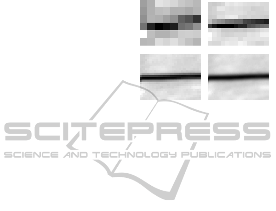
(a) AWS1 100 µm at 280nm (b) AWS1 50 µm at 280nm
(c) AWS1 20 µm at 280nm (d) AWS1 10 µm at 280nm
Figure 2: Exemplary illustration: Four different scan reso-
lutions of black alpaca wool AWS1 at 280 nm.
impact (e.g. squeeze them with tweezers). A com-
plete overview of the used fibers, originating donors
and considered types can be found in the appendix in
8.
Overall, 50 physical fiber specimen are micro-
scopically prepared (5 broad groups × 5 represen-
tatives each × 2 samples per representative). Alto-
gether 16 scans are digitized for each physical sam-
ple (2 consecutive scans × 2 measurement areas × 4
scan resolutions). Summarizing, 800 measurement
results are sensed, whereas only 400 are part of our
experimental test set. Consecutive scans are not con-
sidered in this work.
Every sensor scan is parameterized with an inte-
gration time of 150 ms (illumination duration) and the
measurement head is adjusted manually on the z-axis
(approx. 1 mm height above the specimen). The mea-
sured reflectance spectra is stored 16-bit encoded [0-
65535] for each pixel in the respective scan resolu-
tion. Per pixel 2048 spectral values are measured be-
tween 163 nm and 844 nm in steps of approx. 0.33
nm. Depending on the beforehand adjusted lateral
scan resolution, a finer, larger measurement result is
obtained (scan duration increases as well). Point dis-
tances < 100 µm represent an oversampling due to the
size of the illuminated spot.
The analysis steps of segmentation, feature ex-
traction and BioHash generation are performed by a
scientific software called “SpectroAnalyzer” (see 3),
written in C# (.Net Framework version 4.5).
Image segmentation is realized by applying a
manually selected global threshold to a gray-scale im-
age. Spectral images at 280 nm offer a good contrast
for binarization (see Figure 4(a)). Impurities like dust
or other scan artifacts can be (de)-selected pixel-wise.
As result a binary mask is created and stored for each
SpectralFiberFeatureSpaceEvaluationforCrimeSceneForensics-TraditionalFeatureClassificationvs.BioHash
Optimization
297
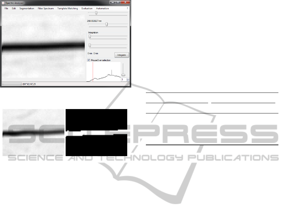
Figure 3: Screenshot of scientific software “SpectroAna-
lyzer”, file opened: 10 µm scan of black alpaca wool ACB1
(a) Raw ACG1 at 280nm (b) Segmented ACG1
Figure 4: Visualization: Segmentation process of gray
acrylic fiber ACG1 at 280nm.
sample (see Figure 4(b)).
As already stated in 3.2, our segmentation approach
consists of a selection of a fixed number of pixels (for
each scan resolution), representing the maximum en-
ergy responses of the segmented fiber area. Neither
pre-processing, nor feature normalization techniques
are applied. Every segmented pixel and the corre-
sponding feature vector is utilized for classification
for both objectives O1.1 and O2.1.
Objective O1.2 and O2.2 require the calculation of
an interval matrix as helper data as well as the gener-
ation of BioHash vectors as actual features. Both are
generated based on mutually exclusive data of equal
size. Thus, this BioHash feature extraction procedure
for O1.2 and O2.2 take place as follows:
Selected pixels of a sample are split into two
equally sized and fully disjoint subsets by using even
pixels and their corresponding feature vectors for IM
calculation and odd ones for BioHash generation.
Consequently, one half of the selected pixels is con-
tributing to the IM calculation and the other half re-
sults in BioHash feature vectors. Thus, we calcu-
late 4 BioHash feature vectors for a scan resolution
of 100 µm and 7, 34, 170 vectors for 50 µm, 20 µm,
10 µm, respectively.
For any further steps the helper data (IM) is dis-
carded and only resulting BioHash feature vectors are
considered for training and classification. Standard
parameterization without local or global interval in-
fluence is applied for each TV = 0 and T F = 1
Our classification basis is also depending on four
different scan resolutions and feature vectors, which
are related to the number of segmented pixels (see 1).
However, every feature space consists of 2048 spec-
tral values, so 2048 attributes form our classification
foundation. The number of classification instances is
calculated by multiplying the segmented amount of
fiber pixel with 100 (50 specimens × 2 measurement
areas).
Table 1: Description of our classification basis.
Scan Property No. Instances
Resolution No. Pixel O1.1/O2.1 O1.2/O2.2
100 µm 8 px 800 400
50 µm 14 px 1400 700
20 µm 68 px 6800 3400
10 µm 340 px 34000 17000
Labelled raw and BioHash feature vectors are clas-
sified using Weka machine learning software (ver-
sion 3.6.8) (Hall et al., 2009). Accuracy and Cohen’s
Kappa are used as quality measure for the classifier
performance. Due to the limited amount of test-data
a tenfold cross validation is applied for testing.
5 RESULTS
All obtained classification results are generated using
Weka (version 3.6.8) (Hall et al., 2009) and rounded
to two digits of precision. Bold printed values display
the best classifier performance in the respective scan
resolution. Classification results are presented in tab-
ular form as follows: correct (cor.), incorrect (incor.)
classified (accuracy), Cohen’s Kappa (Kap.).
5.1 O1 - Identification
A fiber is assigned to the corresponding broad group
(one out of five) based on O1.1 raw spectral (see 2)
and O1.2 BioHash data (see 3). O1.1: As the scan
resolution gets finer the accuracy increases as well.
Rotation Forest achieved the best performance with
one exception at 50 µm. O1.2: The BioHash seems to
improve the overall classification performance, even
on smaller resolutions. SMO and IBk achieve the best
performance for this objective, whereas Naive Bayes
shows the poorest.
VISAPP2015-InternationalConferenceonComputerVisionTheoryandApplications
298

Table 2: O1.1 - Classification results of identification based on raw spectral data.
100 µm 50 µm 20 µm 10 µm
Classifier cor. incor. Kap. cor. incor. Kap. cor. incor. Kap. cor. incor. Kap.
N. Bayes 64.63 35.38 0.56 66.21 33.79 0.58 69.74 30.26 0.62 68.85 31.15 0.61
SMO 87.38 12.63 0.84 91.00 9.00 0.89 96.81 3.19 0.96 98.76 1.24 0.98
IBk 94.75 5.25 0.93 96.79 3.21 0.96 98.91 1.09 0.99 99.70 0.30 1.00
Bagging 82.75 17.25 0.78 88.14 11.86 0.85 93.96 6.04 0.92 96.99 3.01 0.96
R. Forest 94.88 5.13 0.94 96.50 3.50 0.96 99.25 0.75 0.99 99.77 0.23 1.00
JRip 77.50 22.50 0.72 83.71 16.29 0.80 90.88 9.12 0.89 95.48 4.52 0.94
J48 78.88 21.13 0.74 85.29 14.71 0.82 92.15 7.85 0.90 94.61 5.39 0.93
Table 3: O1.2 - Optimized classification results of identification based on BioHash spectral data.
100 µm 50 µm 20 µm 10 µm
Classifier cor. incor. Kap. cor. incor. Kap. cor. incor. Kap. cor. incor. Kap.
N. Bayes 42.00 58.00 0.28 39.71 60.29 0.25 45.15 54.85 0.31 59.42 40.58 0.49
SMO 95.75 4.25 0.95 99.71 0.29 1.00 99.82 0.18 1.00 99.91 0.09 1.00
IBk 99.50 0.50 0.99 98.57 1.43 0.98 99.41 0.59 0.99 99.94 0.06 1.00
Bagging 97.00 3.00 0.96 98.57 1.43 0.98 98.97 1.03 0.99 99.58 0.42 0.99
R. Forest 99.25 0.75 0.99 99.43 0.57 0.99 99.62 0.38 1.00 99.92 0.08 1.00
JRip 89.25 10.75 0.87 94.00 6.00 0.93 98.12 1.88 0.98 99.53 0.47 0.99
J48 95.25 4.75 0.94 92.43 7.57 0.91 98.09 1.91 0.98 99.46 0.54 0.99
5.2 O2 - Individualization
O2.1: Our obtained individualization results resemble
the identification ones (see 4 and 5). Nevertheless, at
100 µm in comparison to O1 our results are a little
bit worse. Yet, at this point it has to be noted that
one out of 25 classes is assigned here. However, Ro-
tation Forest and IBk perform well again. Rotation
Forrest achieved the best overall performance of ob-
jective O2.1 at 10 µm with 99.77% correct assigned
fibers. For objective O2.2, the Bagging classifier was
able to correctly assign every fiber at 50 µm. Be-
sides this, IBk and SMO classify as satisfying as well,
while Naive Bayes performs with low accuracy again.
5.3 O3 - Classification Evaluation
6 and 7 show the classifier performance difference be-
tween BioHash and raw feature data. Negative values
point at a classification performance deterioration of
the BioHash algorithm in comparison to raw spectral
data. An average of all classifier results and Kappa
values of the same column is presented in the last tab-
ular line.
O3.1: as the resolution gets finer the BioHash per-
formance improvement is decreased. Nonetheless, al-
most every classifier accuracy and Kappa is improved,
except for the Naive Bayes. O3.2: In comparison to
O3.1 the average improvement of O3.2 is significantly
higher. The JRip classifier results are increased by
remarkable 37.75% at 100 µm. Similar to O3.1 the
BioHash improvement effect of classifiers with lower
predictive performance is higher (e.g. Bagging, JRip,
J48). On the contrary, the results of the Naive Bayes
learner are getting worse, especially for O3.1.
6 CONCLUSION
We conclude our findings and derive future tasks in
the following section. Our achieved results showed
the optimization influence of the BioHash algorithm.
Nevertheless, the impact is significantly higher at in-
dividualization tasks, which is reasonable because
classification results based on raw spectral data are
already very promising (around 90%). According
to this, the Biometric Hash algorithm is capable of
boosting almost every tested classifier’s accuracy,
without favoring false assignments. Better predicting
classifiers in objective O1.1 and O2.1 are less influ-
enced by the BioHash optimization effect and vice
versa. For the purpose of identification the follow-
ing classifiers performed satisfyingly on our test data:
O1.1 - IBk; Rotation Forrest; O1.2 - SMO, IBk, Bag-
ging, Rotation Forrest, J48. Whereas for individu-
alization our best performing classifiers are: O2.1 -
SMO, IBk, Rotation Forrest; O2.2 - SMO, IBk, Bag-
ging, Rotation Forrest, J48.
It seems to be rather predictable that the overall
performance of the Naive Bayes classifier is low in
comparison to all the others. Unfortunately, the strong
independence assumptions are not fulfilled by our fea-
SpectralFiberFeatureSpaceEvaluationforCrimeSceneForensics-TraditionalFeatureClassificationvs.BioHash
Optimization
299

Table 4: O2.1 - Classification results of individualization based on raw spectral data.
100 µm 50 µm 20 µm 10 µm
Classifier cor. incor. Kap. cor. incor. Kap. cor. incor. Kap. cor. incor. Kap.
N. Bayes 52 48 0.5 52.79 47.21 0.51 53.28 46.72 0.51 49.65 50.35 0.48
SMO 87.75 12.25 0.87 94.00 6.00 0.94 97.44 2.56 0.97 98.19 1.81 0.98
IBk 82.13 17.88 0.81 88.43 11.57 0.88 95.91 4.09 0.96 98.81 1.19 0.99
Bagging 64.25 35.75 0.63 71.64 28.36 0.70 85.28 14.72 0.85 90.74 9.26 0.90
R. Forest 91.13 8.88 0.91 94.21 5.79 0.94 97.79 2.21 0.98 98.80 1.20 0.99
JRip 50.00 50.00 0.48 54.57 45.43 0.53 76.13 23.87 0.75 84.63 15.37 0.84
J48 60.75 39.25 0.59 66.93 33.07 0.66 78.56 21.44 0.78 83.31 16.69 0.83
Table 5: O2.2 - Optimized classification results of individualization based on BioHash spectral data.
100 µm 50 µm 20 µm 10 µm
Classifier cor. incor. Kap. cor. incor. Kap. cor. incor. Kap. cor. incor. Kap.
N. Bayes 61.50 38.50 0.60 48.00 52.00 0.46 56.85 43.15 0.55 60.21 39.79 0.59
SMO 95.00 5.00 0.95 99.57 0.43 1.00 99.79 0.21 1.00 99.87 0.13 1.00
IBk 99.25 0.75 0.99 98.43 1.57 0.98 99.21 0.79 0.99 99.86 0.14 1.00
Bagging 99.25 0.75 0.99 100.00 0.00 1.00 99.18 0.82 0.99 99.43 0.57 0.99
R. Forest 98.50 1.50 0.98 98.57 1.43 0.99 98.88 1.12 0.99 99.81 0.19 1.00
JRip 87.75 12.25 0.87 92.57 7.43 0.92 96.97 3.03 0.97 99.12 0.88 0.99
J48 93.00 7.00 0.93 90.00 10.00 0.90 97.18 2.82 0.97 99.04 0.96 0.99
Table 6: O3.1 - Comparison of raw identification and optimized BioHash classification results.
100 µm 50 µm 20 µm 10 µm
Classifier Cl. imp. Ka. imp. Cl. imp. Ka. imp. Cl. imp. Ka. imp. Cl. imp. Ka. imp.
N. Bayes -22.63 -0.28 -26.50 -0.33 -24.59 -0.31 -9.43 -0.12
SMO 8.38 0.10 8.71 0.11 3.01 0.04 1.16 0.01
IBk 4.75 0.06 1.79 0.02 0.50 0.01 0.24 0.00
Bagging 14.25 0.18 10.43 0.13 5.01 0.06 2.58 0.03
R. Forest 4.38 0.05 2.93 0.04 0.37 0.00 0.15 0.00
JRip 11.75 0.15 10.29 0.13 7.24 0.09 4.05 0.05
J48 16.38 0.20 7.14 0.09 5.94 0.07 4.84 0.06
Average 5.32 0.07 2.11 0.03 -0.36 0.00 0.51 0.01
Table 7: O3.2 - Comparison of raw individualization and optimized BioHash classification results.
100 µm 50 µm 20 µm 10 µm
Classifier Cl. imp. Ka. imp. Cl. imp. Ka. imp. Cl. imp. Ka. imp. Cl. imp. Ka. imp.
Naive Bayes 9.50 0.10 -4.79 -0.05 3.57 0.04 10.56 0.11
SMO 7.25 0.08 5.57 0.06 2.35 0.02 1.68 0.02
IBk 17.13 0.18 10.00 0.10 3.29 0.03 1.05 0.01
Bagging 35.00 0.36 28.36 0.30 13.90 0.14 8.69 0.09
Rot. Forest 7.38 0.08 4.36 0.05 1.09 0.01 1.01 0.01
JRip 37.75 0.39 38.00 0.40 20.84 0.22 14.49 0.15
J48 32.25 0.34 23.07 0.24 18.62 0.19 15.73 0.16
Average 20.89 0.22 14.94 0.16 9.09 0.09 7.60 0.08
ture vectors. Thus, applying the BioHash on objective
O1.2 makes it even worse. The individualization re-
sults O2.2 for this classifier are not affected negatively
in such a degree. Highly sophisticated classifiers like
Bagging, Rotation Forrest or SMO perform well on
the one hand, but a lazy learner like IBk, achieves very
good results on the other hand, too. Nevertheless,
when it comes to computational effort, the k-nearest
neighbor approach of the IBk, with model generation
and evaluation at the same time, is in front. However,
IBk behaves better on the BioHash optimized feature
space. Thus, a resemblance to the BioHash as a tem-
VISAPP2015-InternationalConferenceonComputerVisionTheoryandApplications
300

plate matching approach can be seen since it also uses
a nearest neighbor algorithm.
Furthermore, the FRT sensor is evaluated regard-
ing the suitability for fiber trace acquisition. Scans
with 100 µm resolution are affected the most by the
BioHash optimization capabilities. Nonetheless, clas-
sification results, generated from more detailed scans,
are also improved by applying our BioHash method-
ology. However, we recommend scans with a point
distance smaller than 100 µm (100 µm suitable for
coarse scan, e.g. fiber detection), even though it is
an oversampling with the utilized device. Although,
new and worn fibers can be assigned correctly by our
introduced analysis pipeline, it is not clarified if the
chemical composition or color is the distinguishing
characteristic expressed in our analyzed measurement
data. So the question concerning an individualization
without particular characteristics cannot be answered
conclusively.
6.1 Limitations
Some decisions that were made are accompanied
by limitations. Regarding our test data acquisi-
tion, the working distance between measurement head
and specimen is adjusted manually. Due to the
time-consuming acquisition procedure (between 10s
- 100 µm and 20 min - 10 µm scan) only a limited
amount of test data is evaluated. Concerning the Bio-
Hash algorithm, no parameterization for the inter-
val mapping is evaluated. Neither a tolerance factor
nor a tolerance vector was empirically pre-determined
(both set to default values). Only default parame-
ter settings for all classifiers as well as for the Bio-
Hash are used in our tests. Our evaluated spectral
feature space is not yet analyzed in respect to the
expressed fiber characteristics in our obtained mea-
surement data. Therefore, it needs to be investigated
which physical fiber characteristic (chemical or color
property) is measured and thereby represented in the
spectral data. Nevertheless, our experimental method-
ology was chosen carefully to avoid such side effects.
Furthermore, it could be crucial to analyze the chemi-
cal composition of fibers and their color in order to
evaluate the discriminatory power of individualiza-
tion characteristics.
6.2 Future Work
To strengthen our results that are shown in this paper
a larger amount of experimental data needs to be eval-
uated with fully disjoint sets of training and test data
for the purpose of classification. Besides this, differ-
ent sensor parameterization should be evaluated re-
garding their influence on the classification accuracy
(e.g. working distance, integration time). Will differ-
ent scans of the exact same sample lead to the same
classifier prediction? A feature selection could be per-
formed on our large wavelength range feature space.
Band-pass or -block filters can be applied in order to
emphasize or ignore certain wavelengths (e.g. peaks,
which express certain lamp characteristics). Further-
more, an optimization regarding a suitable BioHash
tolerance factor and vector for the interval mapping
could be potentially useful. A different way of a
BioHash training phase for interval matrix generation
should be designed in order to gain more data for the
BioHash feature generation. To achieve a higher de-
gree of measurement data reproduction-ability, other
procedures of data acquisition should be considered.
Our sampled consecutive scans can be assessed us-
ing a differential imaging approach. Finally, differ-
ent spectroscopic sensors, with transmissively or re-
flectively working principle, should be comparatively
evaluated with our physical specimens.
ACKNOWLEDGEMENTS
The work in this paper has been funded in part by the
German Federal Ministry of Education and Science
(BMBF) through the Research Program under Con-
tract No. FKZ:13N10818. The authors would like to
thank our project partner, the Brandenburg University
of Applied Sciences for the collaborative work and for
the sensor scans, measured with outstanding commit-
ment by Adrienne Thuemler. We also want to thank
the experts from the Berlin and Saxony-Anhalt state
police for the joint discussion and input regarding cur-
rent spectroscopic analysis practice.
REFERENCES
(2000). Standard test methods for identification of fibers in
textiles.
Appalaneni, K., Heider, E. C., Moore, A. F. T., and
Campiglia, A. D. (2014). Single fiber identifica-
tion with nondestructive excitation-emission spectral
cluster analysis. Analytical Chemistry, 86(14):6774–
6780. PMID: 24432828.
Arndt, C., Kraetzer, C., and Vielhauer, C. (2012). First
approach for a computer-aided textile fiber type de-
termination based on template matching using a 3d
laser scanning microscope. In Proceedings of the 14th
workshop on Multimedia and Security, MMSec ’12,
pages 57–66. ACM, New York, NY, USA.
Fries Research & Technology GmbH (FRT) (2010). Data
sheet frt ftr - thin film reflectometer.
SpectralFiberFeatureSpaceEvaluationforCrimeSceneForensics-TraditionalFeatureClassificationvs.BioHash
Optimization
301

Hall, M., Frank, E., Holmes, G., Pfahringer, B., Reutemann,
P., and Witten, I. H. (2009). The weka data min-
ing software: An update. SIGKDD Explor. Newsl.,
11(1):10–18.
Hildebrandt, M., Arndt, C., Makrushin, A., and Dittmann,
J. (2012). Computer-aided fiber analysis for crime
scene forensics. In Bouman, C. A., Pollak, I., and
Wolfe, P. J., editors, Proc. of SPIE 8296, Computa-
tional Imaging X, 829601, volume 8296.
Hildebrandt, M., Makrushin, A., Qian, K., and Dittmann,
J. (2013). Visibility assessment of latent fingerprints
on challenging substrates in spectroscopic scans. In
De Decker, B., Dittmann, J., Kraetzer, C., and Viel-
hauer, C., editors, Communications and Multimedia
Security, volume 8099 of Lecture Notes in Computer
Science, pages 200–203. Springer Berlin Heidelberg.
Houck, M. M. and Siegel, J. A. (2010). Fundamentals of
Forensic Science. Academic Press, 2nd edition edi-
tion.
Inman, K. and Rudin, N. (2001). Principles and Practice of
Criminalistics - The Profession of Forensic Science.
CRC Press.
Jain, A. K. (1989). Fundamentals of Digital Image Process-
ing. Prentice Hall.
Kurabayashi, T., Saitoh, F., Watanabe, N., and Tanno, T.
(2010). Identification of textile fiber by terahertz spec-
troscopy. In Proc: 35th International Conference on
Infrared Millimeter and Terahertz Waves (IRMMW-
THz), pages 1–2.
Millington, K. R. (2012). Diffuse reflectance spectroscopy
of fibrous proteins. Amino Acids, 43(3):1277–1285.
Platt, J. C. (1998). Sequential minimal optimization: A fast
algorithm for training support vector machines. Tech-
nical report, Advances in Kernel Methods - Support
Vector Learning.
Prange, A., Reus, U., Boeddeker, H., Fischer, R., and Adolf,
F.-P. (1995). Microanalysis in forensic science: Char-
acterization of single textile fibers by total reflection
x-ray fluorescence. In Analytical Sciences, volume 11,
pages 483–487.
Stoeffler, S. (1996). A flowchart system for the identifica-
tion of common synthetic fibers by polarized light mi-
croscopy. Journal of Forensic Sciences, 41:297–299.
SWGMAT (1999). Forensic fiber examination guidelines.
Online available: http://www.swgmat.org/Forensic
%20Fiber%20Examination%20Guidelines.pdf.
Vielhauer, C. (2006). Biometric User Authentication for
IT Security - from Fundamentals to Handwriting.
Springer Science+Business Media, Inc.
Vielhauer, C., Steinmetz, R., and Mayerhofer, A. (2002).
Biometric hash based on statistical features of online
signatures. In Pattern Recognition, 2002. Proceed-
ings. 16th International Conference on, volume 1,
pages 123–126.
Witten, I. H., Frank, E., and Hall, M. A. (2011). Data
Mining Practical Machine Learning Tools and Tech-
niques. Elsevier, 3. auflage edition.
APPENDIX
Table 8: Experimental test-set description.
No. Identifier Fiber Type Color Donor
Natural Fibers: Animal Hair - Alpaca Wool
1 AWB alpaca wool beige new wool thread
2 AWBR alpaca wool brown new wool thread
3 AWG alpaca wool green new wool thread
4 AWS alpaca wool black new wool thread
5 AWW alpaca wool white new wool thread
Natural Fibers: Animal Hair - Sheep Wool
6 SWB sheep wool beige used sweater
7 SWG sheep wool gray used sweater
8 SWO sheep wool olive-green used sweater
9 SWR sheep wool red used cardigan
10 SWS sheep wool black used cardigan
Natural Fibers: Plant - Cotton
11 BWW cotton white used shorts
12 BWR cotton red used shorts
13 BWK cotton khaki used shirt
14 BWG cotton light gray used shorts
15 BWS cotton black used T-shirt
Chemical Fibers - Acrylic
16 ACB acrylic blue used knitted cap
17 ACG acrylic gray used knitted cap
18 ACDG acrylic dark gray used knitted cap
19 ACS acrylic black used cap
20 ACW acrylic white used cap
Chemical Fibers - Polyester
21 PEB polyester blue new sewing thread
22 PEG Polyester yellow new sewing thread
23 PER Polyester red new sewing thread
24 PES Polyester black new sewing thread
25 PEW Polyester white new sewing thread
VISAPP2015-InternationalConferenceonComputerVisionTheoryandApplications
302
