
Pedestrian Re-identification
Metric Learning using Symmetric Ensembles of Categories
Sateesh Pedagadi
1
, James Orwell
1
and Boghos Boghossian
2
1
Kingston University, London, U.K.
2
Ipsotek Ltd, London, U.K.
Keywords:
Metric Learning, Categorization, LF.
Abstract:
This paper presents a method for pedestrian re-identification, with two novel contributions. Firstly, each
element in the target population is classified into one of n categories, using the expected accuracy of the
re-identification estimate for this element. A metric for each category is separately trained using a standard
(Local Fisher) method. To process a test set, each element is classified into one of the categories, and the
corresponding metric is selected and used. The second contribution is the proposal to use a symmetrised
distance measure. A standard procedure is to learn a metric using one set as the probe and the other set as the
gallery. This paper generalises that procedure by reversing the labels to learn a different metric, and uses a
linear (symmetrised) combination of the two. This can be applied in cases for which there are two distinct sets
of observations, i.e. from two cameras, e.g. VIPER. Using this publicly available dataset, it is demonstrated
how these contributions result in improved re-identification performance.
1 INTRODUCTION
Pedestrian re-identification is a canonical challenge
for automated analytics systems. It allows systems
to generate hypotheses about the whereabouts of in-
dividuals that encompass a greater extent of space
and time. Person re-identification has been an area
of interest due to its applicability in video surveil-
lance with a camera network involving multiple non-
overlapping cameras. Face recognition technology is
not considered to be applicable in this context, due
to the relatively low resolution and the unconstrained
pose. This variation in pose, illumination and dif-
ferent viewpoints across cameras are the major chal-
lenges in identifying individuals across multiple cam-
eras.
The standard problem definition is to use an un-
seen test set comprising pairs of observations, split
into equal-sized probe and gallery subsets. To evalu-
ate any given technique, it is used to compare each
probe element against the gallery set, ranking the
gallery items in order of similarity. The rank indices
of the correct matches are accumulated to produce an
Cumulative Match Characteristic (CMC), which can
be used to compare different techniques.
The methods proposed by the computer vision re-
search community for person re-identification can be
broadly categorized as being feature, fast matching
and metric learning based. A detailed performance
evaluation of local features which can be used for
person re-identification can be found in (Bauml and
Stiefelhagen, 2011). Histograms were used for iden-
tification and recognition in the early work of Swain
and Ballard (Swain and Ballard, 1990). Franzena et al
(Farenzena et al., 2010) proposed features that com-
bined recurring local color patches with maximally
stable color reqions and histograms. Multiple im-
ages were used to collect histograms with ‘epitome’,
which was defined as a group of stable and recurring
local color patches in the method proposed in (Baz-
zani et al., 2010). A triangulated graph was estimated
on a over segmented image of individuals in (Gheis-
sari et al., 2006). Zhang et al (Zhang and Li, 2011)
proposed the combination of Local Binary Patterns
estimated from non-overlapping regions, with Gabor
and Region Covariance descriptors. Javed et al (Javed
et al., 2005) proposed an illumination variation cor-
rection technique, Inter Camera Brightness Transfer
function (BTF) to address the illumination variation
that usually exists between pairwise cameras.
Fast matching based methods focus on the for-
mat of the descriptor, used to index the observations,
to improve the matching performance. Such tech-
niques require the computation of low dimensional
descriptors for efficient storage. Camillia key-points
are stored in a KD-tree in the method proposed in
(Hamdoun et al., 2008); elsewhere, random forests
are used (Liu et al., 2012) to weight most informative
274
Pedagadi S., Orwell J. and Boghossian B..
Pedestrian Re-identification - Metric Learning using Symmetric Ensembles of Categories.
DOI: 10.5220/0005270602740280
In Proceedings of the 10th International Conference on Computer Vision Theory and Applications (VISAPP-2015), pages 274-280
ISBN: 978-989-758-090-1
Copyright
c
2015 SCITEPRESS (Science and Technology Publications, Lda.)

features from a pool of features; and a layered code-
book is used (Jungling et al., 2011) to encode spatial
information. The recent LDFV proposal (Ma et al.,
2012) employs local descriptors containing location,
intensity, first and second order derivatives, encoded
as Fisher vectors.
The pose of individuals has also been explored
(Aziz et al., 2011; Jungling and Arens, 2011) as a
means to add distinctiveness which is estimated be-
fore the feature extraction process. Multiple obser-
vations (or multi-shot methods) have also proved to
be effective: for example a HoG detector has been
used (Bedagkar-Gala and Shah, 2011) to extract vari-
ous parts of the body. Several other methods (Faren-
zena et al., 2010), (Bazzani et al., 2012) use multi-shot
observations in a semantic segmentation framework.
Other researchers have investigated the possibil-
ity of selecting a discriminative feature set from a
large pool of Haar-like features, using existing itera-
tive learning frameworks. Adaboost is a typical selec-
tion mechanism (Bak et al., 2010); another proposal
is to build an ensemble of weak classifiers (Gray and
Tao, 2008) thereby generating the discriminative fea-
ture set. A number of weak RankSVMs are boosted
(Prosser et al., 2010) using a sampling strategy that
partitions the dataset into overlapping sets.
Person re-identification has also been investigated
as a data association problem, to match and rank ob-
servations from a pair of cameras. Typically, the dis-
tance measures calculated in the original feature space
will not be particularly effective, since multiple ob-
servations of the same individual will lie on a specific
sub-manifold, and Euclidean distances will not dis-
criminate between distances on the same manifold,
and distances of different individuals lying on differ-
ent manifolds. Hence, the requirement for a mapping
to a more used space, for which the associated met-
ric provides an improved discriminative capability,
such that Nearest Neighbour techniques are applica-
ble. Several methods have been proposed recently for
learning this transformation: Dikmen et al proposes
the use of the ‘Large Margin’ Nearest Neighbor with
Rejection (LMNN-R) algorithm (Dikmen et al., 2011)
to learn the most effective metric. Alternatively, a
low dimensional manifold was estimated (Yang et al.,
2011) using kernel based PCA, and SVMs trained on
multi-partitioned data (Kozakaya et al., 2011) can be
used to learn the transformation to a target metric
space. in and the probabilistic distance, PRDC be-
tween features belonging to same and different per-
sons is proposed in (Zheng et al., 2011).
RLPP, a variant of Locality Preserving Projections
(LPP) is estimated over Riemannian manifolds in
(Harandi et al., 2012). Wu et al (Wu et al., 2011) pro-
posed rank loss optimization as a means to improve
the re-identification accuracy. Using constraints in
pairwise difference space, Kostinger et al proposed
learning a metric in (Kostinger et al., 2012) whereas
the person re-identification problem is re-formulated
as a set-based verification task to exploit information
from unlabelled data in (Zheng et al., 2012). PCCA
(Mignon and Jurie, 2012) was proposed to learn a
metric when only a small set of examples are avail-
able. Recently, Rui et al (Zhao et al., 2013b) proposed
the use of dense color histograms and SIFT features
to learn salient and discriminative regions in an un-
supervised manner. The same methodology is then
integrated with RankSVM to add rank constraints for
learning a saliency model in (Zhao et al., 2013a).
The proposed method Symmetrized Ensembles for
Local Fisher, SELF formulates the solution as a data
association problem, drawing upon the above cited
metric learning approaches, with two novel contri-
butions, to provide improved performance on public
benchmark datasets. The proposed method employs
the Local Fisher LF method (Pedagadi et al., 2013),
since its low complexity allows a realtime implemen-
tation that provides relatively good performance.
2 PROPOSED METHOD
The proposed method comprises the following steps,
which create and use a set of categories to train (and
use) a corresponding set of learned metrics. To be
specific, the Local Fisher method is employed, but
any equivalent metric learning method could also be
used. The method for training is as follows:
1. Learn a global distance metric using the Local
Fisher (LF) method, on a training set consisting
of pairs of observations.
2. Use the global metric on the training data to gen-
erate a Cumulative Match Characteristic (CMC).
3. Partition the training set in to n categories, using
n − 1 thresholds applied to this CMC.
4. Using these categories as training sets, learn a
classifier C to categorize future (unseen) observa-
tions into one of n categories.
5. For each category, using the corresponding train-
ing subset, learn reverse category-specific dis-
tance metric i.e a transformation from gallery set
to probe set.
To use the proposed re-identification method on a
test set, these steps are followed:
1. Apply LF metric in to estimate a regular distance
matrix
PedestrianRe-identification-MetricLearningusingSymmetricEnsemblesofCategories
275

2. Classify each of the probe observations in the test
set into one of the n categories.
3. For each probe item in the test set, using the ap-
propriate reverse metrics for its category, calculate
the distances between it and the m observations in
the gallery. Doing so would generate a category
based distance matrix.
4. For each probe in the test set, use a linear com-
bination of the two distance measures to each
gallery element, to produce a rank-order. Use the
Ground Truth to identify the correct gallery ele-
ment in each case, and hence construct the CMC.
2.1 Learning a Global Metric
This section provides a summary of the method em-
ployed to learn a global metric, M
A→B
, with the ob-
jective of minimising the distance (in the transformed
feature space) between different observations a and b
of the same individual. The observations a and b are
members of the probe set A and the gallery set B , re-
spectively. The method is described in greater detail
elsewhere (Pedagadi et al., 2013). A training dataset
is required to ‘learn’ a metric: this comprises two sets
{x
A
1
, x
A
i
, . . . , x
A
m
} and {x
B
1
, x
B
i
, . . . , x
B
m
}, that is, m pairs
of observations about each subject i. The grouping
into sets A and B may be arbitrary, or there may be
some systematic variation in characteristics between
these two sets, e.g. recorded from cameras A and B
having different views or specifications. The vectors
x
A,B
i
represent the original feature sets: these can be
transformed into lower dimensional vectors y
A,B
i
us-
ing a projection P onto the k principle components
y
A
i
= Px
A
i
(1)
and similarly for the {x
B
i
}.
The distance metric M
A→B
is estimated by using
a Fisher learning process with a local aspect, incor-
porating a regularization term to avoid singularities.
This method is explained in more detail elsewhere
(Pedagadi et al., 2013): it is then used to transform
the reduced features as follows:
z
A
i
= M
A→B
y
A
i
(2)
z
B
i
= M
A→B
y
B
i
(3)
The standard application of this transformation is to
rank the true match |z
A
i
− z
B
i
| against all the false
matches, |z
A
i
− z
B
j
|, j 6= i. In addition to ranking un-
seen observations, in the proposed method, this trans-
formation is also used to classify dataset elements into
indicative categories of re-identification accuracy, and
thereby learn two metrics for each category. This is
described in the section below.
2.2 Categories of Re-identification
Accuracy
The CMC curve indicates the range of accuracy with
which a dataset can be re-identified. (Unsurprisingly,
higher accuracy is demonstrated on the training set,
than the test set: this reflects the extent of overtrain-
ing present in the regime.) The CMC is aggregated
from the set of rank results r(1), r(i), . . . , r(n). A re-
sult of r(i) = 1 indicates that the correct match was the
first ranked hypothesis, i.e. a perfect re-identification
result.
This rank result can be used to assign a category
c(i) to each element of the dataset, using κ cate-
gories of accuracy, c
1
, c
j
, . . . , c
κ
. A simple process
can be defined for this purpose, using a set of κ inte-
ger thresholds ρ
1
, ρ
j
, . . . , ρ
κ
, where the first threshold
is always fixed at ρ
1
= 0.
c(i) = max
j
c
j
: ρ
j
< r(i) (4)
In other words, the dataset is partioned into subsets,
such that the first subset contains the elements most
accurately re-identified, the second subset contains
the next most accurate subset, and so on until the least
accurately re-identified subset is labelled with c
κ
. The
set of thresholds {ρ
j
} can be chosen to obtain approx-
imately equal sizes of subsets allocated to each cate-
gory. These can be read off the CMC curve by divid-
ing the cumulative match (y-axis) into equal fractions
and looking up the corresponding rank indices from
the x-axis.
2.3 Prediction of Re-identification
Accuracy
The labels {c(i)} assigned using the method de-
scribed in in Section 2.2 can be used to train a clas-
sifier for re-identification accuracy. The objective for
this classifier is to correctly predict into which seg-
ment of the CMC any (previously unseen) pair of ob-
servations j will fall. In other words, the classifier
will aim to predict the category c( j) that indicates the
likely rank result r( j).
To predict the category of an unseen test vector z
A
,
a training set is used that consists of the reduced fea-
ture vectors {y
A
i
}, and their associated labels {c(i)}.
Both training and test vectors are transformed using
the inclusive Local Fisher projection M
A→B
, as de-
scribed in Section 2.1. It can be noted that this train-
ing set includes only the probe set A, and not the
gallery set A.
A simple ‘nearest neighbour’ method is described
to predict the category of the test vector. The k nearest
VISAPP2015-InternationalConferenceonComputerVisionTheoryandApplications
276

training set vectors to z
A
are recorded, and their cat-
egories are accumulated. The test vector is assigned
that category for which there is the greatest number
of corresponding labels, amongst the k nearest neigh-
bours.
2.4 Category-specific Projections
Once that a category can be estimated for the un-
seen test observation, it is possible to define and em-
ploy category-specific process that may, it is hypoth-
esised, improve the overall re-identification accuracy.
In other words, different transformations can be esti-
mated from the data, to accommodate each category
of input observation (wherein the category is defined
by the expected level of re-identification accuracy).
‘Hard’ cases can be treated differently to ‘easy’ cases.
Thus, category-specific Local Fisher pro-
jection matrices are proposed, i.e. matrices
{M
1
A→B
, . . . , M
κ
A→B
} corresponding to the cate-
gories {c
1
, . . . , c
κ
} each trained in the standard
manner (Pedagadi et al., 2013). This will project the
observation data into a lower dimensional manifold
where the Euclidean distances between observations
reflect the within-class and inter-class designations.
2.5 A Symmetric Distance Measure
The above process is sufficient to define and use a set
of category-specific projection matrices. Experiments
are presented in section 3.1 that demonstrate that this
can contribute to an improvement in re-identification
performance.
Furthermore, a separate innovation can also be
considered. Hitherto, only the projection matrices
M
c
A→B
have been used: the significance of A → B
is that set A is the probe, and set B is the gallery.
This is a reasonable approach, not least because the
standard experimental approach is to maintain this ar-
rangement for the test set.
However, it is worth considering the reverse ar-
rangement, in which set B is the probe and set A
is the gallery. This would enable a corresponding
projection matrix M
B→A
to be trained, along with
the category-specific variants, M
1
B→A
, . . . , M
κ
B→A
. A
working hypothesis is that these projection matrices
may be able to be used alongside the matrices derived
from the original arrangement, to improve the overall
re-identification accuracy.
A simple way to combine these two alternate con-
figurations is to define a distance using a linear combi-
nation of the two respective distances. However, there
is also the opportunity to combine the generic, ‘inclu-
sive’ distance, along with the category-specific vari-
ant. Thus, there are two sets of learned transforma-
tions, M
c
A→B
and M
c
B→A
, that define the metric dis-
tances d
c
A→B
(i, j) and d
c
B→A
(i, j), for the κ categories
c:
d
c
A→B
(i, j) =
M
c
A→B
y
A
i
− M
A→B
y
B
j
(5)
An overall symmetrised distance d
c
i j
can be
defined by taking a linear combination of the
generic distance d
A→B
(i, j) and the category-specific,
reverse-order distance d
c
B→A
(i, j). By convention,
these quantities are scaled with α and 1 − α, respec-
tively:
d
c
(i, j) = αd
A→B
(i, j) + (1 − α)d
c
B→A
(i, j) (6)
Various arguments can be made to justify how α
can be set. Further analysis of the variation in α is
presented in the experiments section.
3 EXPERIMENTAL RESULTS
The proposed method was evaluated on VIPER (Gray
et al., 2007) pedestrian re-identification dataset. The
dataset contains images of individuals as seen from
two cameras. The performance results are reported
as Cumulative match characteristic (CMC), a widely
accepted measure in the field of ranking.
3.1 VIPER
The VIPER dataset is a pedestrian re-identification
dataset containing images of 632 individuals as seen
from two cameras. The images were captured over the
course of one month, making the dataset representa-
tive of a real world video surveillance scenario. The
challenges presented in this dataset include a large
variation in lighting and colour between images of the
same individual in two cameras.
For the performance analysis of the reported
method, the traditional strategy of randomly divid-
ing the dataset into two equal halves is employed.
The feature vector is defined using 8x8 pixel cells, ar-
ranged as a rectangular grid such that 50 percent over-
lap is maintained with each neighbouring cell. The
rectangular grid covers the overall size of the image
which is 128 pixel high and 64 pixels wide. In each
cell, an 8 bin histogram is accumulated for each of
the colour channels of YUV and HSV spaces. As ex-
plained in (Pedagadi et al., 2013), LF metric is esti-
mated by keeping the unsupervised learning of PCA
sub space separate for each of the colour spaces YUV
and HSV. The ‘standard’ metric M
A→B
is estimated
using the training set and the metric dimensionality is
set to 100.
PedestrianRe-identification-MetricLearningusingSymmetricEnsemblesofCategories
277
Two categories of re-identification accuracy are
used (κ = 2), i.e. c
1
and c
2
are ‘easy’ and ‘hard’ cat-
egories, respectively. The metric M
A→B
is then ap-
plied on the training set itself to generate a CMC as
explained in section 2.2. A threshold of 1 is applied
on the rank of the estimated CMC. All probe obser-
vations that contain the correct match at the first rank
are assigned a category of c
1
, and the remainder are
assigned a value of c
2
. The probe and gallery set are
then swapped by retaining the index order for learn-
ing the easy and hard category metrics as discussed in
2.2. The three transformations, M
A→B
, M
1
B→A
, and
M
2
B→A
are estimated, using the first 100 dimensions
of the eigen-transformed feature vectors. This step
concludes the training in the proposed method.
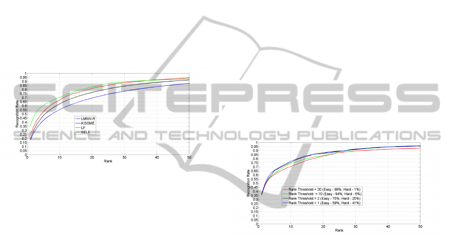
Figure 1: CMC performance for VIPER dataset.
To evaluate the performance, each element i of the
test set is categorised into either c(i) = c
1
(easy) or
c(i) = c
2
(hard) using the nearest training set neigh-
bours defined by the inclusive transformation M
A→B
as explained in 2.3. This category is used to select
the appropriate reverse transformation, i.e. M
c(i)
B→A
.
The distances to the gallery set are calculated using
an evenly weighted sum of the corresponding pairs of
distances, setting α = 0.5.
The proposed method SELF is compared with
several state-of-the-art metric learning methods:
KISSME (Kostinger et al., 2012) , LMNN − R (Dik-
men et al., 2011), eLDFV (Ma et al., 2012) and
LF (Pedagadi et al., 2013). For quantitative analy-
sis, the CMC Fig(1) is computed as an average of
individual CMCs estimated for 100 random trials.
SELF demonstrates good performance amongst all
the methods with a recognition rate improvement of
9.51 percent improvement over eLFDV , 11.9 percent
over LF, 16.27 percent over KISSME and 17.28 per-
cent over LMNN − R.
4 DISCUSSION
Several parameters significantly affect the proposed
method’s performance. The following sections dis-
cuss the variation of these parameters in detail.
4.1 Choice of the Threshold Rank
The choice of the threshold rank discussed in section
2.2 used for categorizing observations into various
levels of difficulty is discussed here. As explained
in section 3.1, the number of categories is set to 2,
easy and hard respectively. The threshold on the rank
is applied on the CMC of the training set for cate-
gorizing observations. Given a training set of 316
observations (half of VIPER dataset’s total observa-
tions), various threshold on rank for categorization
will vary the number of observations in each category.
It is expected that as the threshold on rank increases,
the number of ’easy’ to re-identify observations will
increase and vice-versa for ’hard’ to re-identify cate-
gory. The experiments conducted in this regard also
signify this trend where in as the rank threshold is
set to 1, 2, 10 and 20 consecutively and the resulting
CMC on test set was estimated.
Figure 2: Variation of Rank Threshold on VIPER dataset.
The resulting CMC results Fig(2) for each of the
variation in rank threshold demonstrate decreasing
performance as the percentage of observations avail-
able for hard category reduce as the rank threshold is
increased. For example when rank threshold is set to
1, the number of hard category observations in train-
ing set are 41% of the complete training set while for a
rank threshold of 20, the percentage of hard category
observations is significantly lower at 1%.
4.2 Choice of Category Classifier
A number of different approaches can be employed,
to classify the test set observations into one of the cat-
egories of expected accuracy, as discussed in section
2.3. The experiments reported here consider the case
of κ = 2, effectively ‘easy’ and ‘hard’ categories. It
is reasonable to assume that the overall recognition
accuracy of the proposed method will depend on the
accuracy of the classifier used. To investigate this re-
lation, CMCs are estimated for two type of classifiers.
VISAPP2015-InternationalConferenceonComputerVisionTheoryandApplications
278
One is LF based classifier and the second is a lin-
ear SVM based classifier. On the other hand, a linear
SV M based classifier (Fan et al., 2008) is considered
for the same probe set for categorizing probe obser-
vations into easy and hard categories. The full dimen-
sionality of the feature space is considered during the
construction of the linear SVM classifier.
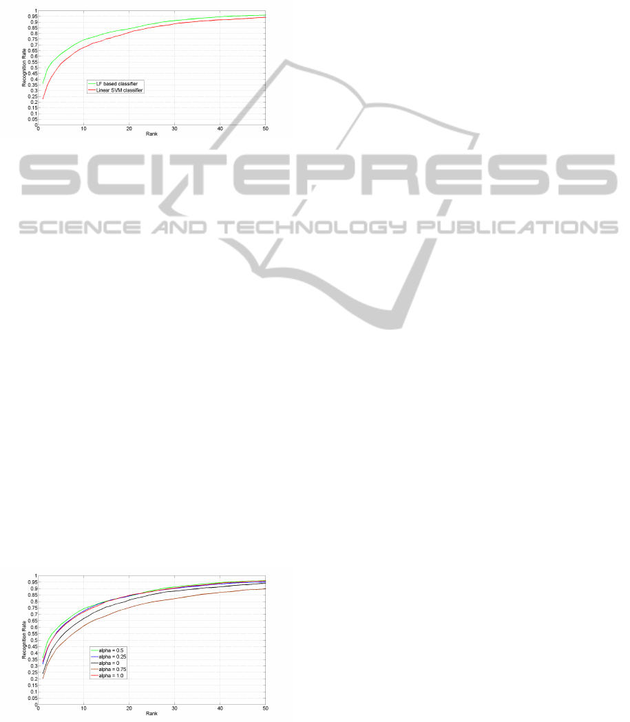
Figure 3: Classifier performance variation on VIPER
dataset.
A comparison in performance was made using the
CMC Fig(3) LF based classifier attains an improved
accuracy of 9% over the linear SV M classifier. This
could be attributed to the fact that LF classifier’s man-
ifold space is much more discriminative due to the
preservation of the local neighbourhood nature of the
data. In the case of linear SVM, the classifier operates
in the high dimensional feature space which could
in itself be highly non-linear in nature. Other types
of metric learning based classifiers can be substituted
that can attain better classification accuracy in future
work.
4.3 Variation of Linear Combination of
Distances
The choice of parameter α introduced in section 2.5
also plays an important role in the recognition accu-
racy of the proposed method. For the case studies in
this context that deals with only two categories of dif-
ficulty, i.e. Easy and Hard, α lies in the range of 0 to
1.
Figure 4: Variation of alpha on VIPER dataset.
If α is set to 1, then the final distance matrix com-
pletely relies on the metric M
A→B
, while setting α = 0
implies that only the category based metrics M
1
B→A
,
M
2
B→A
will be used. In other words, a value of 0 for
α will ensure there is no contribution from global dis-
tance matrix while a value of 1 will neglect the con-
tribution from category based distance metric in the
computation of final distance matrix. This analysis is
conducted by examining the recognition accuracy in
CMC curves Fig(4) as α is varied from 0 to 1. The
observed trend in CMCs demonstrate that there exists
a base line performance which is very similar to that
of normal LF recognition performance when α lies in
the extremity i.e values of 0 and 1. The best recogni-
tion accuracy is achieved when α is set to 0.5, indicat-
ing that equal contributions are made by global metric
and category metrics. As α varies from 0 to 0.5 and
reduces from 1 to 0.5 in reverse, similar variations in
recognition accuracy can be noted.
5 CONCLUSIONS
This paper presented two novel extensions to ex-
isting ‘metric learning’ methods for pedestrian re-
identification. One extension was the introduction
of categories of subject, based on the difficulty of
re-identification, which were used to train category-
specific metric transformations. Another innovation
was the realisation that the role of the datasets used
to learn the transformation can be reversed, hence
making better use out of a given resource of training
data. This two contributions were combined into a
method that demonstrated significant improvements
over other state-of-the-art metric learning methods.
Further investigation into these extensions, e.g. to
increase the effectiveness at higher numbers of cat-
egories and additionally permute the training set vari-
ations, may yield yet more improvements.
REFERENCES
Aziz, K.-E., Merad, D., and Fertil, B. (2011). Person
re-identification using appearance classification. In
ICIAR (2), pages 170–179.
Bak, S., Corvee, E., Bremond, F., and Thonnat, M. (2010).
Person re-identification using haar-based and dcd-
based signature. In Proc. Seventh IEEE Int Advanced
Video and Signal Based Surveillance (AVSS) Conf,
pages 1–8.
Bauml, M. and Stiefelhagen, R. (2011). Evaluation of lo-
cal features for person re-identification in image se-
quences. In Proc. 8th IEEE Int Advanced Video and
PedestrianRe-identification-MetricLearningusingSymmetricEnsemblesofCategories
279

Signal-Based Surveillance (AVSS) Conf, pages 291–
296.
Bazzani, L., Cristani, M., Perina, A., Farenzena, M.,
and Murino, V. (2010). Multiple-shot person re-
identification by hpe signature. In ICPR, pages 1413–
1416.
Bazzani, L., Cristani, M., Perina, A., and Murino, V. (2012).
Multiple-shot person re-identification by chromatic
and epitomic analyses. Pattern Recognition Letters,
33(7):898–903.
Bedagkar-Gala, A. and Shah, S. K. (2011). Multiple per-
son re-identification using part based spatio-temporal
color appearance model. In Proc. IEEE Int Computer
Vision Workshops (ICCV Workshops) Conf, pages
1721–1728.
Dikmen, M., Akbas, E., Huang, T., and Ahuja, N. (2011).
Pedestrian recognition with a learned metric. Com-
puter Vision–ACCV 2010, pages 501–512.
Fan, R.-E., Chang, K.-W., Hsieh, C.-J., Wang, X.-R., and
Lin, C.-J. (2008). LIBLINEAR: A library for large
linear classification. Journal of Machine Learning Re-
search, 9:1871–1874.
Farenzena, M., Bazzani, L., Perina, A., Murino, V., and
Cristani, M. (2010). Person re-identification by
symmetry-driven accumulation of local features. In
CVPR, pages 2360–2367.
Gheissari, N., Sebastian, T., and Hartley, R. (2006). Person
reidentification using spatiotemporal appearance. In
Computer Vision and Pattern Recognition, 2006 IEEE
Computer Society Conference on, volume 2, pages
1528–1535. IEEE.
Gray, D., Brennan, S., and Tao, H. (2007). Evaluating ap-
pearance models for recognition, reacquisition, and
tracking. In 10th IEEE International Workshop on
Performance Evaluation of Tracking and Surveillance
(PETS).
Gray, D. and Tao, H. (2008). Viewpoint invariant pedes-
trian recognition with an ensemble of localized fea-
tures. Computer Vision–ECCV 2008, pages 262–275.
Hamdoun, O., Moutarde, F., Stanciulescu, B., and Steux,
B. (2008). Person re-identification in multi-camera
system by signature based on interest point descriptors
collected on short video sequences. In ICDSC, pages
1–6.
Harandi, M. T., Sanderson, C., Wiliem, A., and Lovell,
B. C. (2012). Kernel analysis over riemannian man-
ifolds for visual recognition of actions, pedestrians
and textures. In Proc. IEEE Workshop Applications
of Computer Vision (WACV), pages 433–439.
Javed, O., Shafique, K., and Shah, M. (2005). Appearance
modeling for tracking in multiple non-overlapping
cameras. In Computer Vision and Pattern Recogni-
tion, 2005. CVPR 2005. IEEE Computer Society Con-
ference on, volume 2, pages 26–33. IEEE.
Jungling, K. and Arens, M. (2011). View-invariant per-
son re-identification with an implicit shape model. In
Proc. 8th IEEE Int Advanced Video and Signal-Based
Surveillance (AVSS) Conf, pages 197–202.
Jungling, K., Bodensteiner, C., and Arens, M. (2011). Per-
son re-identification in multi-camera networks. In
Proc. IEEE Computer Society Conf. Computer Vision
and Pattern Recognition Workshops (CVPRW), pages
55–61.
Kostinger, M., Hirzer, M., Wohlhart, P., Roth, P. M., and
Bischof, H. (2012). Large scale metric learning from
equivalence constraints. In Proc. IEEE Conf. Com-
puter Vision and Pattern Recognition (CVPR), pages
2288–2295.
Kozakaya, T., Ito, S., and Kubota, S. (2011). Random en-
semble metrics for object recognition. In ICCV’11,
pages 1959–1966.
Liu, C., Wang, G., Lin, X., and Li, L. (2012). Person re-
identification by spatial pyramid color representation
and local region matching. IEICE Transactions, 95-
D(8):2154–2157.
Ma, B., Su, Y., and Jurie, F. (2012). Local Descriptors En-
coded by Fisher Vectors for Person Re-identification.
In 12th European Conference on Computer Vision
(ECCV) Workshops, pages 413–422, Italy.
Mignon, A. and Jurie, F. (2012). Pcca: A new approach
for distance learning from sparse pairwise constraints.
In Proc. IEEE Conf. Computer Vision and Pattern
Recognition (CVPR), pages 2666–2672.
Pedagadi, S., Orwell, J., Velastin, S. A., and Boghossian,
B. A. (2013). Local fisher discriminant analysis for
pedestrian re-identification. In CVPR, pages 3318–
3325.
Prosser, B., Zheng, W.-S., Gong, S., and Xiang, T. (2010).
Person re-identification by support vector ranking. In
BMVC, pages 1–11.
Swain, M. J. and Ballard, D. H. (1990). Indexing via color
histograms. In ICCV’90, pages 390–393.
Wu, Y., Mukunoki, M., Funatomi, T., Minoh, M., and
Lao, S. (2011). Optimizing mean reciprocal rank for
person re-identification. In Proc. 8th IEEE Int Ad-
vanced Video and Signal-Based Surveillance (AVSS)
Conf, pages 408–413.
Yang, J., Shi, Z., and Vela, P. A. (2011). Person reidenti-
fication by kernel pca based appearance learning. In
CRV’11, pages 227–233.
Zhang, Y. and Li, S. (2011). Gabor-lbp based region covari-
ance descriptor for person re-identification. In Proc.
Sixth Int Image and Graphics (ICIG) Conf, pages
368–371.
Zhao, R., Ouyang, W., and Wang, X. (2013a). Person re-
identification by salience matching. In IEEE Interna-
tional Conference on Computer Vision (ICCV), Syd-
ney, Australia.
Zhao, R., Ouyang, W., and Wang, X. (2013b). Unsu-
pervised salience learning for person re-identification.
In IEEE Conference on Computer Vision and Pattern
Recognition (CVPR), Portland, USA.
Zheng, W.-S., Gong, S., and Xiang, T. (2011). Person re-
identification by probabilistic relative distance com-
parison. In Proc. IEEE Conf. Computer Vision and
Pattern Recognition (CVPR), pages 649–656.
Zheng, W.-S., Gong, S., and Xiang, T. (2012). Transfer re-
identification: From person to set-based verification.
In CVPR, pages 2650–2657.
VISAPP2015-InternationalConferenceonComputerVisionTheoryandApplications
280
