
Indoor Sensor Placement for Diverse Sensor-coverage Footprints
Masoud Vatanpour Azghandi, Ioanis Nikolaidis and Eleni Stroulia
Computing Science Department, University of Alberta, T6G 2E8, Edmonton, Alberta, Canada
Keywords:
Wireless Sensor Networks, Indoor Localization, Optimization, Sensor Placement, Smart Homes, Genetic
Algorithms.
Abstract:
Single occupant localization in an indoor environment can be accomplished by the deployment of, properly
placed, motion sensors. In this paper, we address the problem of cost-efficient sensor placement for high-
quality indoor localization, taking into account sensors with diverse coverage footprints, and the occlusion
effects due to obstructions typically found in indoor environments. The objective is the placement of the
smallest number of sensors with the right combination of footprints. To address the problem, and motivated
by the vast search space of possible placement and footprint combinations, we adopt an evolutionary technique.
We demonstrate that our technique performs faster and/or produces more accurate results (depending on the
application) when compared to previously proposed greedy methods. Furthermore, our technique is flexible
in that adding new sensor footprints can be trivially accomplished.
1 INTRODUCTION
Because of their low cost, infrared motion sensors
are being used in research and industry for a vari-
ety of localization purposes including military appli-
cations, target tracking, environment monitoring, in-
dustrial diagnostics, etc. One concern in using motion
sensors for localization is their placement. Subopti-
mal placement may result in inefficient usage of the
equipment, and correspondingly, waste of equipment
cost and deployment effort. Pre–deployment simu-
lation to evaluate the anticipated performance of po-
tential deployment alternatives is a useful methodol-
ogy for systematically obtaining high-quality sensor
placements. The question then becomes how to de-
cide which placements to simulate, i.e., how many
sensors should the potential deployment include, of
what type, and where exactly these sensors should
be placed. In principle, a desirable placement should
have the smallest number of contributing sensors (in
order to minimize equipment cost, deployment effort,
and operating energy consumption) at locations such
that the overall space is sufficiently covered and the
target’s location can be inferred with a desirable de-
gree of accuracy and precision.
The work described in this paper builds on our
previous work, in the context of the Smart-Condo
TM
(Boers et al., 2009; Ganev et al., 2011) project, where
we examined placement of same-type sensors, under
a cardinality constraint (i.e., a limited budget of sen-
sors) (Vlasenko et al., 2014) for the purpose of rec-
ognizing the location of an individual in a home en-
vironment. We adopt a similar formulation in this pa-
per. Namely, the formulation includes the represen-
tation of space as a line drawing (floorplan), and the
possible locations for the sensor place are from a set
which is expressed as a (fine) grid of points over the
floorplan.
The placement is assumed to take place on the
ceiling (facing “down”). While alternative place-
ments can be accommodated, experience from prac-
tical deployments has reinforced that ceiling place-
ment is the most convenient for indoor deployments.
Our set of motion sensors include a variety of differ-
ent volumetric shapes, namely a cone, a square based
pyramid, and a rectangular based pyramid. Consid-
ering only orthogonal placement with respect to the
floor the projection of each of these shapes becomes
a disk, a square and a rectangle, respectively. More-
over, the projection of any sensor might be effected by
walls, doors or obstacles around the house depending
on where the sensor is placed (explained more in Sec-
tion 3.2).
Given the above description for the varieties of
sensors we consider, we expand the problem formu-
lation presented in (Vlasenko et al., 2014) to include
the various sensor footprints (from a finite set of foot-
prints) and to determine the optimal number of sen-
25
Vatanpour Azghandi M., Nikolaidis I. and Stroulia E..
Indoor Sensor Placement for Diverse Sensor-coverage Footprints.
DOI: 10.5220/0005273700250035
In Proceedings of the 4th International Conference on Sensor Networks (SENSORNETS-2015), pages 25-35
ISBN: 978-989-758-086-4
Copyright
c
2015 SCITEPRESS (Science and Technology Publications, Lda.)

sors (not just their placement). The immediate impli-
cation of this more general problem formulation is a
significantly enlarged search space, due to increased
number of possible combinations of placements and
footprints. We address the increase in complexity us-
ing genetic algorithms (GAs). Evolutionary methods,
based on GAs, are frequently employed to explore
large problem spaces in order to identify high-quality
solutions. Our sensor placement problem naturally
belongs to this category. The GA technique elabo-
rated in this paper outperforms the greedy algorithm
in (Vlasenko et al., 2014) in two different aspects.
First it efficiently delivers placements with acceptable
coverage accuracy. For example, we have noted that it
reaches 94.81 percent coverage after just 50 seconds
of execution on an off-the-shelf personal computer.
Second, it delivers placements with higher-accuracy
when efficiency is not a factor. It is able to eventually
reach coverage of 100, whereas the greedy algorithm
can do no better that 98.58 percent.
The remainder of this paper is organized as fol-
lows. In Section 2 we review earlier relevant research
in the same area. Section 3 presents details of our
mobility and sensor coverage model, as well as the
objective function. Section 4 provides a comprehen-
sive discussion of the GA methodology in the context
of our problem, and its parameters. Section 5 presents
simulation results. Finally, we conclude with a sum-
mary of the contributions of this work and some fu-
ture plans in Section 6.
2 RELATED WORK
The sensor placement problem is relevant to many
wireless sensor network (WSN) applications. Kang,
Li, and Xu (Kang et al., 2008) use a virus coevolution-
ary parthenogenetic algorithm (VEPGA) to optimize
sensor placement in large space structures (i.e., por-
tal frame and concrete dam) for modal identification
purposes. They concluded that their method outper-
forms the sequential reduction procedure. Rao and
Anandakumar (Rao and Anandakumar, 2007), also
addressing the sensor placement problem in large-
scale civil-engineering structures, developed a solu-
tion based on particle swarm optimization, another
evolutionary technique. Poe and Schmitt adopt a GA
approach to sensor placement for worst-case delay in
minimization (Poe and Schmitt, 2008). Comparing
their results against a exhaustive and a Monte-Carlo
method, they found out that these methods serve as an
upper and lower bound, respectively. Their method is
a fast and near-optimum solution for optimized place-
ment. These papers show that evolutionary methods
are preferred over the exhaustive search approaches.
However none of them consider as an objective that
of optimizing the number of sensors placed.
Yi, Li and Gu (Yi et al., 2011) compared evolu-
tionary methods for sensor placement and described a
generalized genetic algorithm (GGA) approach for a
predefined number of sensors. According to them the
GGA can get better results than the simple version
of the GA. They also describe a number of different
exhaustive and evolutionary methods to sensor place-
ment.
As we have already mentioned, the work concep-
tually closest to the method described in this paper is
our own previous work (Vlasenko et al., 2014) also
conducted in the context of the Smart-Condo
TM
and
aiming at inexpensive placements for high-accuracy
localization of a individual in a home environment.
The greedy approach of (Vlasenko et al., 2014) iden-
tified sensor locations one at a time, resulting in ex-
ploring a large number of potential locations and, in
some cases, requiring a large amount of time. Our
method adopts evolution-based techniques to address
exactly these shortcomings.
3 MOBILITY AND SENSOR
COVERAGE MODEL
In this section we detail the mobility and coverage
models and we introduce the terminology, notation,
and definitions (Table 1) used in the remaining of the
study.
3.1 Basics of Localization
In order to improve localization accuracy, coverage
areas of the sensors are allowed to overlap. By having
the sensor coverage areas overlap the detection areas
will be reduced because the space is segmented into
new, smaller, polygons defined by the intersection of
the coverage areas. We consider as location of the
individual to be the center of mass of the polygon oc-
cupied by the individual. To illustrate this, Figure 1
is presented. In this figure A12 is the new polygon
that has been created as a result of the overlap of the
coverage areas A1 and A2. A12 has the least amount
of localization error among the regions (because R3
is less than R1, R2, and R4).
With respect to representation conventions, we
can consider each polygon (or, more generally, over-
lap area) to be defined by a specific signature signi-
fying the sensors that are “on” when an individual is
in that polygon. The signature can be represented by
SENSORNETS2015-4thInternationalConferenceonSensorNetworks
26

Table 1: Table of notation.
Symbol Definition
c
i
Coverage utility at point i
v
i
Heat-map value at point i
c
max
Maximum desired coverage score
(c
i
)
t(c
max
) Threshold value
A
s
Points in space covered by sensor s
D
s
Points in space that are “seen
through” the doorway by sensor s
p
s→o
Probability of detection at point o
by sensor s
p
door open
Probability of doors being open
K Budget of sensors
P
Z
o
Probability of detection at point o
by the sensors in set Z
C Chromosome
λ
C
Coverage percentage metric of
chromosome C
F
C
Fitness function for chromosome C
f
Z
Collective information utility
a series of 1s and 0s. If the e
th
motion sensor cov-
ers the polygon, its value of the signature at position
e will be 1, otherwise it is set to 0. For example in
Figure 1 each of the four regions have distinct signa-
tures which are (1, 0, 0), (0, 1, 0), (1, 1, 0) and (0, 0, 1)
for A1, A2, A12 and A3, respectively. The signature
also represents the sensor readings that we will get if
a person is present in the corresponding region.
Trying to find good combinations of sensors to
overlap in certain “important” areas brings complica-
tions too. In Section 5 we show how our proposed
method handles overlaps, and places sensors where
their usefulness is maximized.
3.2 Sensor Coverage Model
As mentioned in our introduction section, walls,
doors and obstacles around the house can restrict sen-
sor footprints. Figure 2 presents an example where
two sensors (marked with green) with originally rect-
angular footprints (depicted with blue lines) are re-
stricted because of obstruction by walls (thick black
lines) and doors (painted in yellow). Some parts of
the polygon fall “behind” a door and the sensor may
cover these areas if the door is open, otherwise the
door restricts the sensor’s projection even further. The
probability of doors being open (p
door open
) directly
A3
A2
A1
A12
R1
R12
R2
R3
Figure 1: Example overlapping sensor coverage areas.
translates into probability of detection in the afore-
mentioned parts of the polygon.
A sensor’s coverage model is:
p
s→o
=
1, if o ∈ A
s
\D
s
p
door open
, o ∈ D
s
0, otherwise
(1)
In this equation z is a point in space, A
s
is the set
of points sensor s covers, and D
s
is a set of points seen
by the sensor through the doorway. A
s
is represented
by:
A
s
: {a
1
, a
2
, . . . , a
kA
s
k
} (2)
For our experiments we will set p
door open
to 0 in
order the avoid complexity. Therefore, we can rewrite
our coverage model, which now becomes a boolean
1
coverage model, as in Equation 3.
p
s→o
=
(
1, if o ∈ A
s
0, otherwise
(3)
If all of the sensors in the set of sensors Z cover
o, the joint sensing probability at that specific point is
(Wang et al., 2006):
P
Z
o
= 1 −
∏
s∈Z
(1 − p
s→o
) (4)
3.3 Mobility Model
In this research, we adopt the environment model
developed in (Vlasenko et al., 2014). We consider
a floorplan and a corresponding “heat-map” created
through observation of the paths traversed by an in-
dividual in this space over time. Figures 3 and 4
1
In most cases, as in our evaluation section, this will be
a “sharp” probability, i.e., either 1 or 0, but the formulation
is applicable to general coverage probabilities.
IndoorSensorPlacementforDiverseSensor-coverageFootprints
27
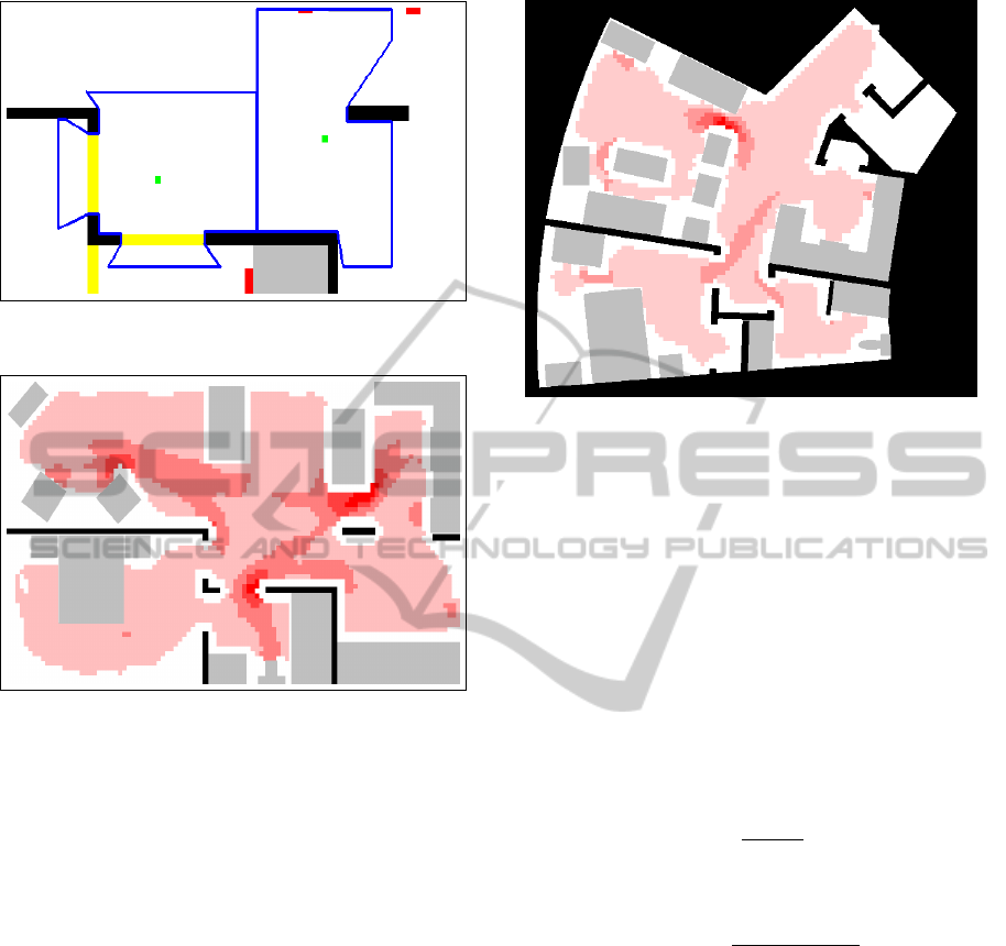
Figure 2: Real shape of sensor coverage projections
(Vlasenko et al., 2014).
Figure 3: Coverage utility heat-map of a person walking in
the Smart-Condo
TM
.
show such floorplans with the heat-map represented
as various intensities of the same colour. The (approx-
imation of this) heat-map can be constructed without
a-priori observations of the occupant, but solely by
knowing the points of interest (e.g. locations in the
environment that form the origin/destination of an oc-
cupant’s paths).
The points of interest must include all potential
destinations in order to cover important areas. Failing
to doing so, will result in data loss and system defi-
ciency. There are various parameters regarding how
to produce the heat-map, and depending on the oc-
cupant, different configurations can be adopted. In
cases were the user tends to choose more random and
unusual paths to traverse, the corresponding param-
eter(s) can be altered to accommodate exactly this.
For more information on how to produce the heat-map
please refer to (Vlasenko et al., 2014).
The heat-map is produced only once, at the pre-
deployment phase. It is at this phase that all the
planning has to be completed. After the sensors are
mounted on the ceiling, redeployment is consider-
ably expensive and time consuming. Thus, we should
make sure that the quantity of sensors in need agree
Figure 4: Coverage utility heat-map of a person walking in
the Independent Living Suit (ILS).
with our cost/accuracy trade-off, and that the place-
ment is optimal.
Next, using the two-dimensional heat-map that
contains N points of interest, (x
1
, y
1
), . . . , (x
N
, y
N
),
where each point has an information utility of v
i
we
construct a coverage utility map (with the same di-
mensions) which is the mapping of intensities from
the heat-map into numerical values. This is done
using a configurable application-specific parameter
called c
max
that indicates the upper bound of values
in the coverage utility map. Equations 5 and 6 show
how the translation between heat-map values (v
i
) and
coverage utility values (c
i
) are calculated.
c
i
=
v
i
t(c
max
)
(5)
Here, c
max
is the maximum desired coverage
score.
t(c
max
) =
max
i∈{1,...,N}
v
i
c
max
(6)
The coverage utility map will be used throughout
the rest of the study, mainly during the optimized sen-
sor placement.
3.4 Objective Function
Given the notation given in Table 1, the placement
problem can be formulated as follows:
Given (a) the coverage utility map and (b) K, the
set of sensors available, where k K k≤ N, the objec-
tive is to find the combination of sensors, Z, that max-
imizes the collective information utility:
f
Z
=
N
∑
i=1
(P
Z
i
.c
i
) (7)
SENSORNETS2015-4thInternationalConferenceonSensorNetworks
28

4 THE EVOLUTIONARY MODEL
GA solutions are represented as a population of chro-
mosomes, where each chromosome consists of genes.
In our model, the genes are a sensor’s type and its
location. In each evolution, new, and hopefully im-
proved, solutions are developed by applying a number
of different operators on the population. The criterion
for deciding whether a particular chromosome is bet-
ter than another is defined through a fitness function,
also known as the cost function. The classical GA
methodology that we use defines the following steps:
• Start. Generate an initial random population of
chromosomes representing potential problem so-
lutions, which in our case is sensor combina-
tions. Section 4.1 discusses the encoding of sen-
sor placements as chromosomes and the construc-
tion of the initial population.
• Loop. Create a new population by:
– selecting a percentage of the current population
as parents, and performing crossover to pro-
duce new offsprings,
– performing mutation of the new offsprings,
– applying elitism, i.e., including the new off-
springs in the new population but reducing the
population to its original size, keeping only the
best solutions for the next iteration.
Section 4.2 discusses the process of population re-
newal.
• Termination Check. If an end condition has been
reached,
– return the best solution in the current popula-
tion,
– else, go to Loop.
Section 4.3 discusses the termination conditions
of our method.
We note that the GA methodology requires a num-
ber of parameters for its configuration, which must be
designed taking into account the specifics of the prob-
lem domain. A list of these parameters is given in
Table 2.
4.1 Chromosome Encoding
Each chromosome in the population contains a num-
ber of genes. In the context of our sensor placement
problem, genes are sensors with coverage models in-
troduced in Section 3.2. A chromosome is therefore
represented by a set of sensors:
C : {s
1
, s
2
, . . . , s
kCk
} (8)
Table 2: GA parameters.
Parameter Description
m Population size
u Number of children produced in
each iteration
n Number of sensors in each initial
chromosome
max Maximum number of sensors that
each solution can have (k K k)
p
c
The probability of crossover for the
parents
p
m
The probability of mutation on each
child
l Number of iterations for the whole
process
By combining equation 4 and 3, we can conclude
that P
C
o
= 1 whenever there is at least one sensor in C
that covers o.
In order to evaluate the performance of a solution
found by the genetic algorithm, we divide the chro-
mosomes collective information gain (calculated ac-
cording to Equation 7) by the summation of positive
coverage utility values. This will give a metric that
we call the coverage percentage metric, formulated
as follows:
λ
C
=
∑
N
i=1
(P
C
i
.c
i
)
∑
N
i=1
c
i
≥0
(c
i
)
∗ 100% (9)
In the Start step, we have to create the initial pop-
ulation for the algorithm to use as its first evolution.
This is done by randomly creating m chromosomes,
i.e., sensor placement solutions. The initial length
of the chromosomes must be set to a value less than
or equal to a user-specified upper bound called max
i.e., (n ≤ max).
4.2 Selection, Crossover, Mutation and
Elitism
To produce children two parents must be selected for
a crossover procedure. The parents are chosen ran-
domly from the population, according to a selection
percentage also known as the crossover probability,
(p
c
). For example, if the population consists of 100
chromosomes, and p
c
= 0.2, then approximately 20
parents are randomly chosen to participate. From the
chosen parents, two parents are randomly selected to
create two children. A second parameter, u, decides
the total number of children that will be produced in
IndoorSensorPlacementforDiverseSensor-coverageFootprints
29

each iteration. We continue the procedure until we
have all u children.
We use the “cut and splice” crossover method
(Banzhaf et al., 1998). In this method, the crossover
point for each parent is chosen separately and ran-
domly. As shown in Figure 5, the first part of the first
parent and the second part of the second parent are
used to construct the genes in the first child, and the
rest construct the second child. Figure 5 shows how
cut and splice is performed to produce two children
from two parents. This crossover method leads to off-
springs with different chromosome lengths, which in
our case implies different numbers of sensors placed.
As we are seeking the number of sensors to use, as
well as the sensor locations, this method helps achieve
this. In addition, throughout the whole process of the
GA, chromosome lengths must remain less than or
equal to max.
Random Position in the Chomosome
Parents
Children
Figure 5: “Cut and splice” crossover method for producing
children chromosomes.
Once u children chromosomes have been pro-
duced through the parent-population crossover, ac-
cording to the mutation probability (p
m
), they might
be mutated. The chromosome mutation operation that
we use in our experiments is called a uniform muta-
tion (Banzhaf et al., 1998), which involves randomly
choosing a gene from the chromosome and perform-
ing the mutation operation on that gene. For this, we
either use relocating the sensor to a new random loca-
tion or we change its type, for example, turn its cov-
erage footprint from a disk to a square.
The last step of this phase involves adding the new
children in the population, and selecting the best chro-
mosomes from the combined population for the next
iteration so that the population cardinality always re-
mains stable. This selection is accomplished through
the fitness function.
The fitness of each chromosome is evaluated ac-
cording to the following three criteria. Sensors should
cover as much heat as possible. Sensors are penalized
for covering “restricted” areas, i.e., areas known to
not require coverage. For example sensors should not
be placed directly on top of a table, simply because
people don’t tend to walk there. Finally, the number
of contributing sensors should be minimized, there-
fore shorter chromosomes are preferable to longer
chromosomes. In order to capture these three crite-
ria, we have formulated the fitness function to be:
F
C
= w1 ∗
N
∑
i=1
(P
C
i
.c
i
) − w2 ∗
kCk
∑
i=1
k A
s
i
k (10)
Where w1 and w2 are fixed values, P
C
i
can be com-
puted using equation 4. Here, because the c
i
for points
in the restricted area is negative, the second criterion
is embedded in the first summation.
4.3 The Termination Criterion
In principle, the evolutionary process terminates if (a)
the maximum number of iterations or execution time
has been reached, or (b) the average fitness of the pop-
ulation does not change over a certain number of evo-
lutions, or (c) 100% accuracy is achieved. When the
genetic algorithm terminates, the best solution in the
current population is returned as the final solution.
5 SIMULATION AND RESULTS
The evolutionary process described above is con-
trolled by the parameters listed in Table 2. As it is
a convention for users of evolutionary algorithms, pa-
rameter tuning needs to be performed based on ex-
perimental comparisons on a limited scale (Smit and
Eiben, 2009). We follow this requirement by fine-
tuning the GA model parameters on a simple artificial
scenario. In the heat-map of Figure 6, the overlap-
ping footprints of several sensors are shown. The dif-
ferent footprint shapes correspond to three different
sensor types; the first type projects a square footprint
(edge = 175 points); the second type projects a rect-
angle (length = 200 and width = 150 points); and the
third type projects a disk (radius = 100 points). The
darker the colour, the higher the significance of the
area, i.e., the higher the utility of the area. The envi-
ronment shown in this simple heat-map consists of 6
different regions to be covered by the sensors, and the
ideal solution should place exactly 6 sensors of the
right types in exactly the right locations. Given this
desired solution, we proceeded to identify the param-
eter configuration that results in the solution at hand.
Because of the implicit randomness of the evolu-
tionary GA process, we cannot predict the exact re-
sulting amounts for coverage percentage. So, the ex-
periments
2
conducted in this section are tested mul-
tiple times (i.e., 50 times), and the average is taken.
2
All experiments are run on Mac OS X, Processor: 1.7
GHz Intel Core i5, Memory: 4 GB 1600 MHz DDR3, plat-
form: Java.
SENSORNETS2015-4thInternationalConferenceonSensorNetworks
30
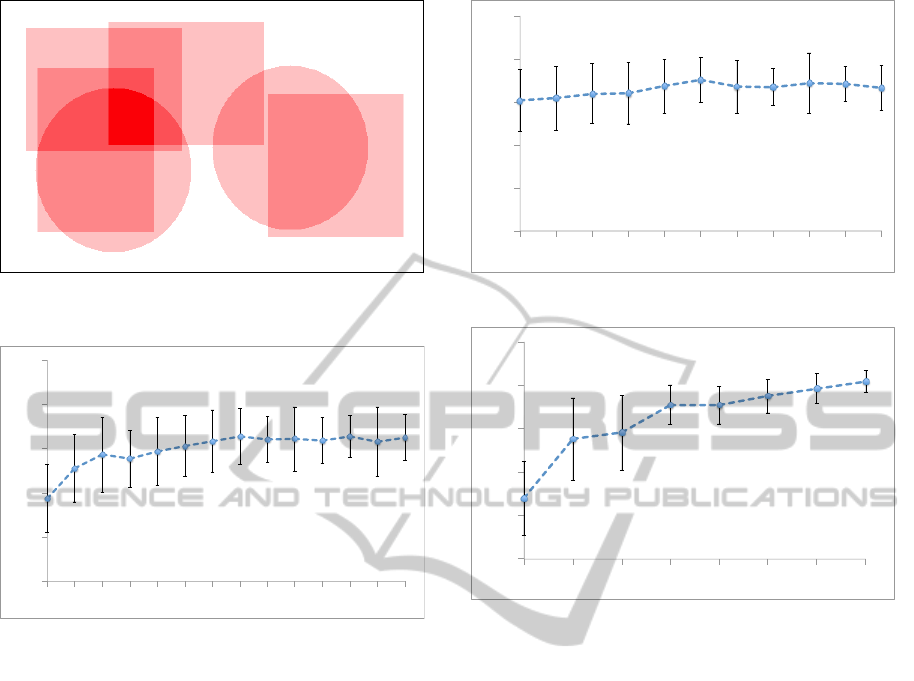
Figure 6: Artificial input with 6 overlapping regions to
cover.
80#
84#
88#
92#
96#
100#
0.02# 0.06# 0.1# 0.3# 0.5# 0.7# 0.9#
Figure 7: Coverage percentage for different values of p
c
.
To configure the algorithm parameters, we started
by optimizing p
c
, with the following initial settings:
m = 50, n = 10, u = 50, l = 50 and p
m
= 0.2. Fig-
ure 7 shows how the coverage percentage changes
for different values of p
c
. Lower p
c
values result
in lower accuracy. This is because, when there is
little crossover in the evolutionary process, the po-
tential parents are less likely to pair with each other
to produce better solutions. On the other hand, a
high crossover probability also threatens accuracy,
because good subsets of sensors inside the chro-
mosomes have a high risk of getting involved in a
crossover procedure and being separated from each
other; in these cases, the good subset, which should
have been passed to the next generation of chromo-
somes, is lost. We notice that the coverage percentage
at p
c
= 0.4 yields the best result. We used this value
for the remainder of the experiments and proceeded
to select p
m
through the experiments shown in Figure
8.
As p
m
increases, more mutations occur and, as a
result, the diversity of the chromosomes increases.
However, too much mutation may result in los-
ing good chromosomes generated through crossover.
Based on the data of Figure 8, p
m
was set to 0.5 for
80#
84#
88#
92#
96#
100#
0# 0.1# 0.2# 0.3# 0.4# 0.5# 0.6# 0.7# 0.8# 0.9# 1#
Figure 8: Coverage percentage for different values of p
m
.
80#
84#
88#
92#
96#
100#
5# 10# 20# 50# 100# 200# 500# 1000#
Figure 9: Coverage percentage for different values of l.
the rest of the experiments.
Figures 9, 10 and 11 show the impact of l, m and u,
respectively. According to Figure 9, higher number of
iterations lead to better coverage percentages. Also,
as Figure 10 suggests the value of m should be set to
be the same as u, which in this case is 50. In Figure
11, we note that increasing the value of m (which is
equal to u) will result in higher accuracy. This is be-
cause, more children are produced in each iteration,
increasing the likelihood of finding a better solution.
Further, as the number of iterations increases, the like-
lihood of identifying a better solution increases since
more of the solution space is explored.
However, the downside to increasing m, u and l is
that execution time will also increase. So the question
becomes how to decide the tradeoff between m, l and
accuracy versus time consumption.
To answer this question we experimented with dif-
ferent configurations of m during different time pe-
riods. As shown in Figure 12 a larger population
size results in better accuracy, given the same amount
of execution time. Note that, because more execu-
tion time is consumed to produce children through
crossover in each iteration, there will be fewer iter-
ations in total.
In addition to running the same algorithm multiple
IndoorSensorPlacementforDiverseSensor-coverageFootprints
31
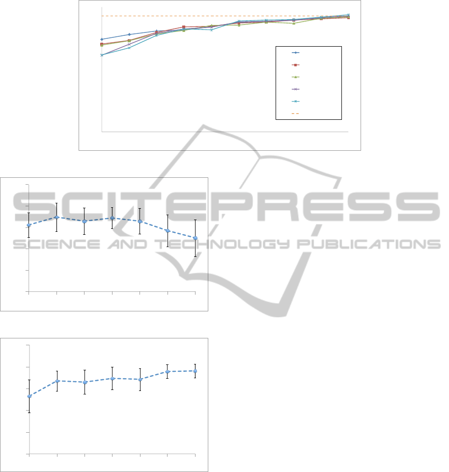
80#
84#
88#
92#
96#
100#
50# 100# 250# 500# 750# 1000# 1250# 1500# 1750# 1974#
m=100#
m=200#
m=300#
m=400#
m=500#
Greedy#
Figure 12: Results from GA for different values of m.
80#
84#
88#
92#
96#
100#
5# 10# 25# 50# 100# 250# 500#
Figure 10: Coverage percentage for different values of m.
80#
84#
88#
92#
96#
100#
10# 25# 50# 75# 100# 150# 200#
Figure 11: Coverage percentage for different values of u.
times, we also illustrate a logarithmic trend line func-
tion in order to visualize how different configurations
of the GA are performing. The trends in Figure 13 in-
dicate that although m = 500 performs slightly worse
than m = 100 at the beginning, it catches up and fi-
nally exceeds the accuracy achieved with m = 100. In
conclusion, the process of parameter fine-tuning re-
ported in this section produced the following param-
eter configuration: m = 500, u = 500, p
c
= 0.4 and
p
m
= 0.5. When m is higher than 500, results deteri-
orate because the time spent in each iteration on pro-
ducing children increases and in a given amount of
time the algorithm cannot perform enough iteration
to achieve acceptable results.
5.1 Comparison Against the Greedy
Method
Let us now compare our GA method against the
greedy algorithm by (Vlasenko et al., 2014). In the
greedy method, sensors are placed one after the other,
in a location which optimizes the additional “heat”,
i.e., utility, covered. Once a sensor is placed, the heat
in the area covered by the sensor is reduced, since
gaining more localization accuracy in a given area
is becoming increasingly less useful as the area gets
covered. This procedure continues until the desired
number of sensors has been reached. It is important to
note here that, in the greedy method (Vlasenko et al.,
2014; Wang et al., 2006), the number of sensors to
be placed is assumed to be decided a-priori, based on
the cost that can be afforded. Near-optimal results are
guaranteed in this method when certain types of sen-
sors are used (Vlasenko et al., 2014). Although re-
alistic, this problem formulation does not address the
cases where the budget is flexible and the users desire
to explore the cost/accuracy tradeoff. Another fun-
damental shortcoming of the greedy method is that it
consumes exponentially more processing time as the
types of available sensors increase.
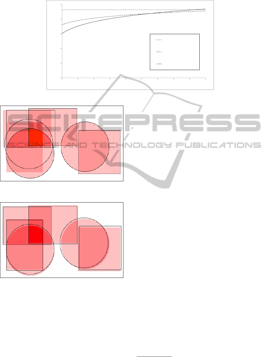
Running the greedy algorithm on the simple heat-
map of Figure 6 always returns the same result of
98.58 percent coverage, after an average time of 1974
seconds. Figure 13 shows that after approximately
1800 seconds the GA surpasses the greedy method.
The greedy does not reach 100 percent accuracy with
the simple case heat-map, because it fails to exactly
match every area with the right sensor (Figure 14);
SENSORNETS2015-4thInternationalConferenceonSensorNetworks
32
80#
84#
88#
92#
96#
100#
50# 100# 250# 500# 750# 1000# 1250# 1500# 1750# 1974#
Greedy#
Log.#(m=100)#
Log.#(m=500)#
Figure 13: Trend lines shown for m = 100 and m = 500.
Figure 14: Sensor placement on a simple case heat-map
with the greedy method.
Figure 15: Sensor placement on a simple case heat-map
with the GA method.
it always starts by covering the highest-utility area,
i.e., the darkest area in the heat-map, and gets stuck
in a local optimum. This phenomenon does not hap-
pen with the genetic algorithm. The GA can get even
100 percent accuracy thanks to its ability to find the
best combination of sensors and not focusing on one
at a time (Figure 15). Although the process may take
time for very high accuracy (i.e., 37333.55 seconds
for 99.81%) but in time critical applications, it can
achieve very high accuracy in short time periods. Ac-
curacy as high as 94.81 % can be reached within the
first 50 seconds.
In order to compare the two methods more real-
istically, we use the two complicated and larger scale
heat-maps, shown in Figures 3 and 4. The scale of the
Smart-Condo
TM
heat-map is 629 × 1060 points and
for the ILS it is 573×651 points. Moreover, the value
of c
max
is set to 4 while producing these heat-maps. It
is noteworthy that the data reported throughout the re-
mainder of this section for the GA is the average of 10
runs.
The comparison methodology here is to first see
how the greedy method is preforming with a desig-
nated budget of sensors and mark its coverage per-
centage (calculated using equation 9) for that budget
as the “desired accuracy”. After that, we give the GA
the same budget and see how fast we can achieve cov-
erage percentages higher than or equal to the desired
accuracy.
In the first experiment conducted, we only use one
type of sensor footprint, the rectangle. Say the bud-
get for covering the ILS is 15 sensors, we would like
to know how much coverage each method achieves
having this budget. It turns out that greedy can get
81.48% coverage percentage in 466.7 seconds. This
value becomes our desired value, that the GA aims to
reach. The GA can achieve this accuracy in just 41.5
seconds on average.
Now, let us use a sensor set consisting of more
than one type of sensor. In the second experiment we
will use a budget of 5 squares, 5 disks, and 5 rectan-
gles (all with the same sizes as before). The same pro-
cedure as in the first experiment is adopted to fill ta-
bles 3 and 4 which show the results for both methods
when dealing with heat-maps 3 and 4, respectively. In
addition, we record the fitness (calculated according
to Equation 10) of the solution as well as the average
3
Number of sensors.
IndoorSensorPlacementforDiverseSensor-coverageFootprints
33

Table 3: Comparison of different methods in the Smart-Condo
TM
layout.
Desired Accuracy (%)
Greedy GA
nos
3
time (s) nos time (s) Average Cost Best Cost σ of Cost
74.29 10 3725 10 185 11933.41 12104.76 49.73
76.82 11 4231 11 275 12744.75 12873.20 44.36
79.93 12 4622 12 391 13313.95 13450.34 53.05
83.69 13 5023 13 387 14401.83 14488.54 47.51
84.50 14 5380 14 372 14389.32 14467.30 45.90
85.25 15 5572 15 348 14453.41 14595.90 51.05
Table 4: Comparison of different methods in the ILS layout.
Desired Accuracy (%)
Greedy GA
nos time (s) nos time (s) Average Cost Best Cost σ of Cost
72.45 10 643 10 56 2442.19 2487.82 16.55
73.77 11 741 11 35 2313.08 2432.68 34.65
76.80 12 837 12 52 2433.45 2504.76 22.44
77.60 13 912 13 62 2461.45 2529.08 26.86
79.43 14 967 14 58 2442.21 2557.78 31.65
80.80 15 996 15 50 2406.02 2524.48 28.05
and standard deviation of chromosome fitness in the
population in which that solution was found (namely
solution cost, average cost, and cost STD).
According to these tables, the GA reached the de-
sired accuracy checkpoint with the same budget of
sensors in considerably less time. Comparing the
results from experiments one and two, we notice
that increasing sensor types affects the greedy’s time
consumption substantially, while increasing the GA’s
only slightly.
The GA can continue beyond this point and find
even better solutions which brings us to our third and
final experiment. In this experiment, again we get
back to only having 15 rectangles and want to see
how much accuracy we can achieve if we let the GA
consume the same amount of time that the greedy
has used. The GA reaches an average coverage per-
centage of 83.55% and shows is superiority when is
comes to hitting high accuracy, too.
6 CONCLUSION
Sensor placement can greatly impact the effective-
ness of sensor-based systems. In our work, in the
context of sensor-based indoor localization, we de-
veloped an evolutionary technique for sensor place-
ment. Our simulation experiments demonstrate that
our method achieves excellent coverage utility (close
to 100%) when time efficiency is not a factor; it also
delivers acceptable accuracy for applications that are
time sensitive. An important feature of our method is
that it does not require an a-priori number of sensors
as input, which is the case with an earlier greedy algo-
rithm developed by our group for this problem. Fur-
thermore, although a larger number of sensor types
tends to increase the run-time of the greedy algorithm,
it does not affect the genetic algorithm described in
this paper.
In the future, we plan to design a hierarchical
framework in the context of which to embed our al-
gorithm. The core idea is to decide sensor locations
for each utility level, starting from the highest level
and progressively descending to lower levels.
We also plan to extend the localization algorithm
with additional information sources, such as dead-
reckoning for a more accurate estimation of the per-
sons location, while this person moves between the
sensor regions.
ACKNOWLEDGEMENTS
This work has been partially funded by IBM, the Nat-
ural Sciences and Engineering Research Council of
Canada (NSERC), Alberta Innovates - Technology
Futures (AITF), and Alberta Health Services (AHS).
SENSORNETS2015-4thInternationalConferenceonSensorNetworks
34

REFERENCES
Banzhaf, W., Francone, F. D., Keller, R. E., and Nordin, P.
(1998). Genetic Programming: An Introduction: on
the Automatic Evolution of Computer Programs and
Its Applications. Morgan Kaufmann Publishers Inc.,
San Francisco, CA, USA.
Boers, N. M., Chodos, D., Huang, J., Gburzynski, P., Niko-
laidis, I., and Stroulia, E. (2009). The smart condo:
Visualizing independent living environments in a vir-
tual world. In Pervasive Computing Technologies for
Healthcare, 2009. PervasiveHealth 2009. 3rd Interna-
tional Conference on, pages 1–8. IEEE.
Ganev, V., Chodos, D., Nikolaidis, I., and Stroulia, E.
(2011). The smart condo: integrating sensor networks
and virtual worlds. In Proceedings of the 2nd Work-
shop on Software Engineering for Sensor Network Ap-
plications, pages 49–54. ACM.
Kang, F., Li, J.-j., and Xu, Q. (2008). Virus coevolution
partheno-genetic algorithms for optimal sensor place-
ment. Advanced Engineering Informatics, 22(3):362–
370.
Poe, W. Y. and Schmitt, J. B. (2008). Placing multiple
sinks in time-sensitive wireless sensor networks us-
ing a genetic algorithm. In Measuring, Modelling and
Evaluation of Computer and Communication Systems
(MMB), 2008 14th GI/ITG Conference-, pages 1–15.
VDE.
Rao, A. R. M. and Anandakumar, G. (2007). Optimal
placement of sensors for structural system identifica-
tion and health monitoring using a hybrid swarm in-
telligence technique. Smart materials and Structures,
16(6):2658.
Smit, S. K. and Eiben, A. E. (2009). Comparing parameter
tuning methods for evolutionary algorithms. In Evolu-
tionary Computation, 2009. CEC’09. IEEE Congress
on, pages 399–406. IEEE.
Vlasenko, I., Nikolaidis, I., and Stroulia, E. (2014). The
smart-condo: Optimizing sensor placement for indoor
localization. Systems, Man, and Cybernetics: Sys-
tems, IEEE Transactions on, PP(99):1–1.
Wang, Q., Xu, K., Takahara, G., and Hassanein, H.
(2006). Wsn04-1: deployment for information ori-
ented sensing coverage in wireless sensor networks.
In Global Telecommunications Conference, 2006.
GLOBECOM’06. IEEE, pages 1–5. IEEE.
Yi, T.-H., Li, H.-N., and Gu, M. (2011). Optimal sensor
placement for structural health monitoring based on
multiple optimization strategies. The Structural De-
sign of Tall and Special Buildings, 20(7):881–900.
IndoorSensorPlacementforDiverseSensor-coverageFootprints
35
