Using Inertial Data to Enhance Image Segmentation

Knowing Camera Orientation Can Improve Segmentation of Outdoor Scenes

Osian Haines, David Bull and J. F. Burn

University of Bristol, Bristol, U.K.

Keywords:

Vision Guided Locomotion, Segmentation, Image Interpretation, Scene Understanding, Inertial Sensors,

Oculus Rift, Mobile Robotics.

Abstract:

In the context of semantic image segmentation, we show that knowledge of world-centric camera orientation

(from an inertial sensor) can be used to improve classiﬁcation accuracy. This works because certain structural

classes (such as the ground) tend to appear in certain positions relative to the viewer. We show that orientation

information is useful in conjunction with typical image-based features, and that fusing the two results in

substantially better classiﬁcation accuracy than either alone – we observed an increase from 61% to 71%

classiﬁcation accuracy, over the six classes in our test set, when orientation information was added. The

method is applied to segmentation using both points and lines, and we also show that combining points with

lines further improves accuracy. This work is done towards our intended goal of visually guided locomotion

for either an autonomous robot or human.

1 INTRODUCTION

Locomotion is fundamental to the survival of humans

and most other land-dwelling animals, in order to ﬁnd

food, escape danger, or ﬁnd mates, for example. One

of the primary senses used to guide locomotion is vi-

sion, enabling animals to perform complex tasks such

as avoiding obstacles, route planning, adjusting to

different terrains and building cognitive maps (Patla,

1997), which would be impossible with other senses.

This has inspired many applications in computer vi-

sion and robotics, which also attempt to use vision

to guide vehicles – either wheeled or legged – over

rough terrain using visual sensors (see for example

(DeSouza and Kak, 2002; Lorch et al., 2002)).

However, another sense available to animals is

from the vestibular system, allowing both relative ac-

celeration and absolute orientation (with respect to

gravity) to be perceived (Angelaki and Cullen, 2008).

This is combined with other senses, such as vision,

and is essential for the accurate balance required for

more agile motions. Interestingly, it has been sug-

gested that the central nervous system dynamically

controls the relative importance of visual and vestibu-

lar signals (Deshpande and Patla, 2007), and that

vestibular sensing may have a larger effect when vi-

sion is impaired. Vestibular sensing is also able to

ameliorate effects due to head motion when ﬁxating

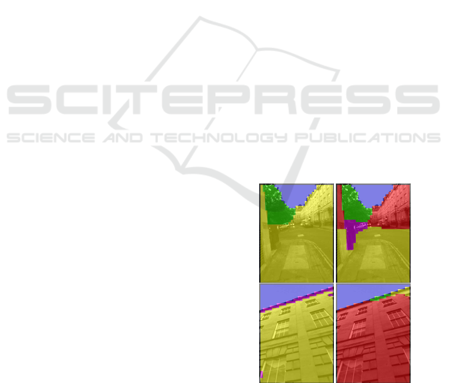
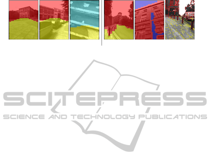
Figure 1: Typical results of our algorithm, showing how

segmentation results using only vision (left) can be im-

proved by taking into account the camera orientation (right).

In both examples knowledge of the camera orientation

avoids misclassifying vertical walls as ground (yellow). See

Fig. 7 for full colour legend. All images are best viewed in

colour.

on an object (Virre, 1996), and its absence causes se-

vere problems in interpreting visual information.

The use of orientation information in interpreting

scene content has been less well studied in the context

Haines O., Bull D. and Burn J..

Using Inertial Data to Enhance Image Segmentation - Knowing Camera Orientation Can Improve Segmentation of Outdoor Scenes.

DOI: 10.5220/0005274000210032

In Proceedings of the 10th International Conference on Computer Vision Theory and Applications (VISAPP-2015), pages 21-32

ISBN: 978-989-758-090-1

 2015 SCITEPRESS (Science and Technology Publications, Lda.)

of mobile robotics however, and is something which

we believe can be put to good use alongside vision.

This is based on the observation that different types

of surface or structure are more likely to be observed

when the camera is facing in different directions: for

example, a camera pointing straight ahead is unlikely

to see the ground in the top half of the image; or a

camera pointing straight downward is very unlikely

to be looking at the sky.

In this paper we show that by using information

about the real-world orientation of a camera obtained

from an inertial sensor, it is possible to improve the

performance of algorithms designed to segment im-

ages into distinct semantic/structural regions, with the

aim of facilitating autonomous navigation through ur-

ban environments – see for example Fig. 1.

While vision is a suitable sensing modality for

such tasks, most solutions focus on using only vi-

sual features. While the location of a point/region in

an image has previously been used to alter likelihood

of predicting certain geometric classes (Hoiem et al.,

2007), to our knowledge the orientation of the camera

itself has not been used to facilitate segmentation in

this way.

Visual navigation is an important topic in robotics,

where the ability to navigate through unknown en-

vironments without human guidance is essential for

tasks such as disaster relief and search-and-rescue

(Kleiner and Dornhege, 2007), planetary exploration

(Maimone et al., 2007), or for self-driving cars

(Dahlkamp et al., 2006).

On the other hand, algorithms such as ours have

the potential to be used to guide humans, as we ex-

plore in this work. We do this primarily because a hu-

man makes a convenient test-bed for evaluating vision

guidance algorithms without the constraints of robot

locomotor capability, and give a useful proxy for how

well robots might be guided. Moreover, such algo-

rithms could also be applicatied as navigation aids for

the visually impaired, where recovering the structure

of a scene is important (Brock and Kristensson, 2013;

Tapu et al., 2013). This paper uses as an example the

goal of designing an algorithm able to guide a human

through an urban environment while wearing a head-

mounted display, through which the result of our seg-

mentation is shown.

The next section discusses related work in the

ﬁeld. A brief overview of our method is given in

Section 3, followed by Section 4 which describes the

data acquisition process. Section 5 gives full details of

how our algorithm works. We then present extensive

results and examples in Section 6, before concluding

in Section 7.

2 RELATED WORK

Combining inertial sensors with computer vision al-

gorithms has been known to improve performance in

a variety of tasks. One of these is visual simultaneous

localisation and mapping, in which the pose of a cam-

era with respect to a map, and the unknown map itself,

must be recovered while it is being traversed. Since

inertial sensors provide an estimate of heading inde-

pendent of that derived from the image stream, these

estimates can be fused to improve robustness (N

utzi

et al., 2011), and help to mitigate scale drift (Pini

et al., 2007). A rather different example from (Joshi

et al., 2010) uses inertial information for blur reduc-

tion, by using estimates of the camera’s motion de-

rived from inertial sensor during an exposure to guide

deconvolution.

More related to our application are tasks such as

segmenting an image into geometrically consistent

regions (Hoiem et al., 2007) and segmenting road

scenes into areas which are driveable or hazardous

(Sturgess et al., 2009). The former uses the position

of a segment within the image as a feature during clas-

siﬁcation, so that the expectation that the sky is near

the top of the image, for example, is learnt from data

– although in this work the camera is assumed to be

in an upright position with no roll. (Sturgess et al.,

2009) and more recently (Kundu et al., 2014) show in-

teresting examples of combining visual segmentation

with 3D information, which respectively use features

extracted from a point cloud to help classify objects

in road scenes, and fuse 2D segmentations and point

clouds to semantically label structure in 3D. While the

orientation of the camera may effect the result via the

3D map, this is not directly investigated, and further-

more is estimated from the image stream itself. Use

of 3D information in the form of depth data is also

useful in semantic segmentation (Gupta et al., 2014).

The use of inertial data for terrain classiﬁcation

was investigated by (Sadhukhan et al., 2004). Rather

than use knowledge of gaze direction to guide seg-

mentation, the inertial data themselves are used as

features to encode the vehicle vibration and accelera-

tions for different terrains, in order to predict the ter-

rain type which the vehicle is currently traversing.

While these show interesting uses of information

not directly present in the image to aid labelling, they

are not making use of the information potentially

provided by the camera orientation itself. Similarly,

while some of the above mentioned works use inertial

data to aid vision tasks, this is generally in a purely

geometric sense, and they have not exploited the rele-

vance to semantic attributes in the image. We investi-

gate ways to do this in the following sections.

VISAPP2015-InternationalConferenceonComputerVisionTheoryandApplications

3 OVERVIEW

In this paper we present an algorithm able to take

a single image with associated 3D orientation, mea-

sured with an inertial measurement unit (IMU), as in-

put, and produce a segmentation of the image into

distinct regions, corresponding to classes relevant to

the task of locomotion. The classes used are: ground

(walkable), plane (non-walkable, usually vertical),

obstacle (non-walkable and not planar), stairs, fo-

liage, and sky (coloured yellow, red, magenta, cyan,

green and blue respectively in all examples). These

were chosen as a reasonably minimal set of necessary

classes to facilitate locomotion through different en-

vironments. The reason we use more than two classes

(simply walkable/non-walkable) is to give more in-

formation to the human (or equivalently, robot) being

guided – for example, stairs can be traversed, but with

caution; foliage may be walkable but may require a

different gait; and a sky region should be interpreted

very differently from an impending obstacle, despite

the fact neither facilitate locomotion. Of course, our

algorithm is not speciﬁc to the classes we use.

To demonstrate the use of orientation in enhanc-

ing segmentation, we developed a relatively simple

means of classifying and segmenting images. We seg-

ment each image by describing a grid of points with

a collection of feature vectors, comprised of visual

and orientation information. These are used to predict

the most likely class for the point, using a pre-trained

classiﬁer. Since each point is classiﬁed independently,

this initial segmentation exhibits much noise. To mit-

igate this, we use a Markov random ﬁeld algorithm

to enforce the assumption of smoothness. With this

framework we show that fusing visual and orientation

information can substantially improve segmentation

accuracy over using either alone.

We also show that using both visual and orienta-

tion features improves performance when classifying

lines in the image. As above, these are described with

a combination of vision and orientation features, plus

features encoding some properties of the line itself.

Finally, we show that combining the results from both

point and line classiﬁcation can improve performance

over either in isolation.

The result of our method is a segmentation of the

image, comprised of sets of contiguous points with

the same classiﬁcation. This is not a per-pixel seg-

mentation, due to the resolution of the grid we use, but

every pixel in the image is covered, and every pixel is

used for the description. As shown in Fig. 1, this is

able to divide the image into regions appropriate for a

navigation task.

4 DATA ACQUISITION

To develop and evaluate the algorithms in this paper,

we gathered long video sequences (totalling around

90 minutes of footage) using an IDS uEye USB 2.0

camera

ﬁtted with a wide-angle lens (approximately

80° ﬁeld of view). This provides images at a resolu-

tion of 640 ×480, at a rate of 30 Hz.

Our aim is to use this method to guide humans

through outdoor environments. Therefore, all our data

are gathered from a camera mounted on the front of

a virtual reality headset, worn by a person travers-

ing various urban environments. While walking, the

subject sees only the view through the camera. This

was done so that the data are as close as possible to

what would be observed in a real application – both

in terms of height from the ground and viewing an-

gle, but also the typical movements and gaze direc-

tions made by a person wearing such a headset, with

somewhat limited visibility.

The hardware we used for this was the Oculus

Rift

(Dev. Kit 1), which has a large ﬁeld of view and

sufﬁciently high framerate (up to 60 Hz). The cam-

era was mounted sideways, so that the images have a

portrait orientation – this is because the view for each

eye is higher than it is wide. We correct for barrel dis-

tortion introduced by the lens to produce an image ap-

proximating a pinhole camera, using camera parame-

ters obtained with the OpenCV calibration tool.

To gather orientation information we used the in-

ertial sensor built into the Oculus Rift. This com-

prises a three-axis accelerometer, gyroscope and mag-

netometer, which are combined with a sensor fusion

algorithm to give estimates of orientation in a world

coordinate frame at 1000 Hz. We retrieve the orienta-

tion as three Euler angles, and discard the yaw angle

(rotation about the vertical axis), since in general this

will not have any relationship to semantic aspects of

the world. Conversely, pitch and roll are important

since they encode the camera pose with respect to the

horizon line, and thus whether the camera is looking

up/down or is tilted. This has an inﬂuence on the like-

lihood of different classes being observed.

From these videos, a subset of frames are chosen

manually for labelling, either for training/validation

or testing. They are divided into disjoint regions, built

from straight-line segments. Each region is assigned

a ground truth label from our set of classes. This is by

nature a subjective task, since image content is often

ambiguous, but the labelling is as consistent as possi-

ble. Some truly ambiguous regions are not labelled,

en.ids-imaging.com

www.oculus.com

www.docs.opencv.org

UsingInertialDatatoEnhanceImageSegmentation-KnowingCameraOrientationCanImproveSegmentationofOutdoor

Scenes

Figure 2: Example ground truth – the manual labelling of

regions (left) and ground truth segmentation (right).

which are omitted from all training and testing.

Examples of ground truth data can be seen in Fig.

2. The labelling is independent of the points and

lines which are later created in the image. We also

show ground truth segmentations derived from these,

in which a grid of points has been assigned labels ac-

cording to the the underlying ground truth (where the

blockiness due to the grid is clearly visible). This

is the best possible segmentation, against which we

evaluate our algorithms in Section 6.

5 CLASSIFICATION AND

SEGMENTATION

In this section we describe the process by which

an image is segmented, according to either the vi-

sual features, orientation features, or both; and where

these features are created in regions surrounding grid

points, detected lines, or both. An overview of the

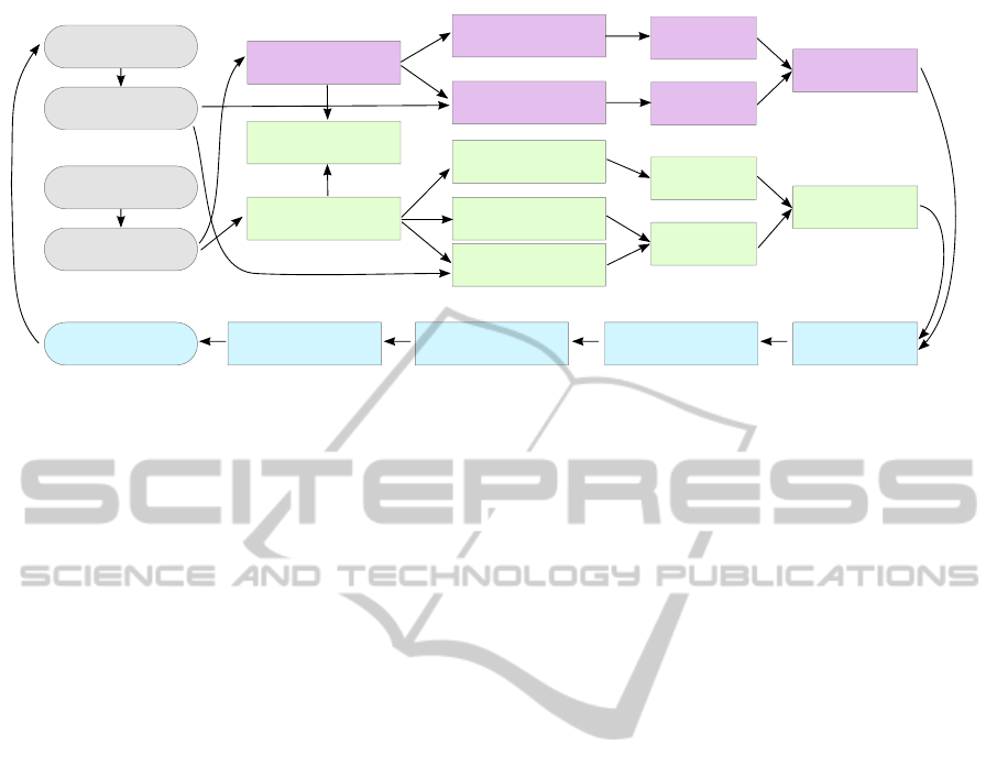
whole system is presented in Fig. 3.

5.1 Features

To describe a point, we build feature vectors from the

pixels in a square patch surrounding the point. We use

two types of visual feature: histograms of gradients,

and colour histograms.

Histograms of gradients are used to represent the

texture of the patch. The image is convolved with gra-

dient ﬁlters in the x and y directions, to obtain at each

pixel gradient responses g

and g

. For each pixel in

a patch we calculate θ = tan

−1

and m =

+ g

which are the gradient angle and magnitude respec-

tively. These are used to build the gradient histogram

by quantising the angle into bins, and weighting the

contribution to each bin by the magnitude. Rather

than creating a single orientation histogram for each

patch, we follow the example of (Haines and Calway,

2012) and create four separate histograms for each

quadrant of the patch, and concatenate them together

in order to encode richer structure information. This

is similar to the way HOG descriptors are built from

multiple cells (Dalal and Triggs, 2005), but without

the overlapping blocks.

Colour has also been shown to be beneﬁcial when

classifying and segmenting images (Hoiem et al.,

2007; Kr

ahenb

uhl and Koltun, 2011). The colour

features we use are histograms built in HSV space,

which combine a histogram of quantised hue values,

weighted by the saturation (since the saturation repre-

sents the degree to which the hue is relevant), and a

separate histogram of the intensity values, to encode

the distribution of brightnesses within the patch.

We shall henceforth refer to the above as ‘vision

features’. The other type of features are the ‘orien-

tation features’. To compute these, we use the pitch

and roll values from the Oculus Rift IMU, each nor-

malised to the range [0, 1]. In addition to these, the

feature vector contains the position in the image of

the point (normalised by the image size). This is im-

portant, since otherwise the orientation feature would

be the same for all points in the image: it is the inter-

action between image position and camera orientation

which gives rise to cues of different types of structure

at different locations in the image.

5.2 Line Regions

An alternative form of the algorithm uses a set of

lines detected in the image. This is done in order to

represent high-frequency image content, and distinc-

tive texture and colour occurring over discontinuities,

which would be missed by the much smaller point

features. To detect lines we use the LSD line seg-

ment detector

(Von Gioi et al., 2010). The regions

are created around these lines, extending along their

length and covering a region of ﬁxed width on either

side (we discard lines under 6 pixels long and 3 pix-

els wide (LSD gives a width value for each line) since

these are likely to be noise).

Line regions too are endowed with both visual and

orientation features. In order to create a description

better suited to lines, for both gradient and colour we

create pairs of histograms, from the pixels in rectan-

gular regions either side of the line, and concatenate

Code available at www.ipol.im/pub/art/2012/gjmr-lsd

VISAPP2015-InternationalConferenceonComputerVisionTheoryandApplications

Create points

Create vision

features

Create orientation

features

Detect lines

Assign points

to lines

Create vision

features

Create orientation

features

Classify

Combine

MRF

Extract Connected

Components

Create graph

Segments

Image

Orientation

(pitch and roll)

Camera

Oculus Rift

Classify

Combine

Create line-shape

features

Figure 3: Block diagram showing how the system as a whole works. The different algorithms discussed in this work corre-

spond to all or some of this. The ‘combine’ blocks can be interpreted as applying meta-learning, or concatenating features

before classiﬁcation, as appropriate.

them. Thus, the gradient descriptor has half the di-

mensionality compared to the point case, while the

colour descriptor is twice as long.

We also add a line shape descriptor, which com-

prises simply its length, width, and orientation in the

image, each appropriately normalised. Finally, we use

the same orientation descriptor, using the line’s mid-

point and the pitch and roll of the camera as above (we

will refer to these together as the orientation features

unless otherwise stated). The use of these features

separately and together is evaluated in Section 6.

In order to combine lines with the rest of the seg-

mentation, we assign points to lines if they lie within

the region enclosed by the line feature (a point may

be assigned to multiple lines). It is this assignment of

points to lines which later allows line classiﬁcations

to be transferred to points for segmentation; similarly,

the ground truth label of a line is obtained via the

points, whose label in turn comes from the marked

ground truth regions (thus a line’s label vector is the

mean label vector of all points inside the area used to

describe it).

5.3 Classiﬁcation

Having extracted features for all points and lines in

our training set, each being paired with a ground truth

label, we train a set of classiﬁers, with which we can

then predict labels for points and lines in new images.

For learning and prediction, we represent each label

as a 1-of-K vector (for the K = 6 classes), where di-

mension k is 1 for class k, and zero otherwise. The

outputs of the classiﬁers, after normalising to sum to

1, are treated as estimated probabilities for each class.

The classiﬁer we use for this work is multivariate

Bayesian linear regression (Bishop, 2006), chosen be-

cause it is both fast to train, and very fast to evaluate

for a new input. It is similar to standard regularised

linear regression, except that the optimal value for the

regularisation parameter can be chosen directly, under

the assumption that the data have a Gaussian distribu-

tion. Since it is multivariate regression (predicting the

K dimensions of the label vector), an M × K weight

matrix is learnt, for M data. Prediction with the linear

regressor is simply a matter of multiplying the fea-

ture vector by the weight matrix. Rather than the raw

feature vector – which would allow for learning only

linear combinations of the inputs – we use fourth or-

der polynomial basis functions.

5.4 Combining Information

We can easily run the algorithm using points (P) or

lines (L) with either vision (V) or orientation (O) fea-

tures in isolation. This leads to the four baseline meth-

ods (denoted P-V, P-O, L-V and L-O respectively,

where L-O combines both orientation and line-shape

features as discussed above). The main theme of this

paper is to combine information from multiple fea-

ture types (vision/orientation) and from different im-

age entities (points/lines), which we describe here.

When classifying points, we can combine the fea-

tures in one of two ways. First and most obviously, we

simply concatenate the vision and orientation features

into one longer feature vector, and train/test with this

(algorithm P-VO-Cat). Or, we train separate classi-

ﬁers for the two feature types, and combine them af-

terwards. This is achieved by concatenating the out-

put K-dimensional label vectors from each classiﬁer

for a point and treating this as a new feature vector.

This is input to a second round of classiﬁcation, the

output of which is another K-d label vector, represent-

UsingInertialDatatoEnhanceImageSegmentation-KnowingCameraOrientationCanImproveSegmentationofOutdoor

Scenes

ing the ﬁnal probability estimate for each class. This

process is known as ‘meta-learning’ (or sometimes

‘stacked generalisation’) (Bi et al., 2008). To train the

meta-classiﬁers, we run the classiﬁers whose outputs

we wish to combine on all points in the training data,

to gather example outputs. These predicted label vec-

tors are concatenated (to make the ‘meta-features’),

and paired with the known ground truth label for each

point to train the meta-learner. We refer to this algo-

rithm as P-VO-Meta.

The above can also apply to line regions, i.e. we

can combine line features either by concatenation

or meta-classiﬁcation (L-VO-Cat and L-VO-Meta).

However, we cannot combine points with lines by

simply concatenating their features, because the point

and line features are created over different areas. In-

stead, we again use meta-learning, applied at the

points. Each point which lies in at least one line re-

gion is assigned the mean label vector from all lines

in which it lies (again normalised to sum to 1). Then a

ﬁnal meta-classiﬁer is trained using the predicted fea-

tures from the points and lines as inputs, to predict the

ﬁnal label vector assigned to the point.

There are still two ways in which this could be

done, depending on how the features were combined

for the entities: either we concatenate the results of P-

VO-Cat and L-VO-Cat to make the meta-feature (PL-

VO-Cat); or use meta-classiﬁers for everything, and

concatenate the outputs of all predicted vectors from

P-V, P-O, L-V and L-O into a meta-feature, which

we call PL-VO-Meta. In either case, we need to deal

with points which are not in any lines: for PL-VO-Cat

we simply use the existing result of P-VO-Cat; for PL-

VO-Meta we train yet another meta-classiﬁer, which

fuses the results of only P-V and P-O, i.e. fall back

to P-VO-Meta (the converse is not necessary, since

there are no points belonging to lines without their

own classiﬁcations). The performance of all of these

combinations is compared in Section 6.

5.5 Segmentation

The result of any of the above algorithms is a set of

points in the image, each having a predicted label

vector, from which we choose the most likely class

assignment as the dimension with the highest value.

Since each point is classiﬁed individually, there is no

guarantee that neighbouring points will have similar

labels, even if they belong to perceptually similar re-

gions of the image; this is especially true when using

line regions, as adjacent points may be assigned to

different lines.

To address this, we follow what has become fairly

standard practice in such tasks (Delong et al., 2012)

and formulate the problem as a Markov random ﬁeld

(MRF). This allows us to choose the best label for

each point according to its observation (i.e. classiﬁ-

cation result), while also incorporating a smoothness

constraint imposed by its neighbours.

We create a graph connecting all the points in the

image – this is simply a grid connecting a point to its

4-neighbours. The aim when optimising a MRF is to

maximise the probability of the conﬁguration of the

ﬁeld (i.e. an assignment of labels to points); this is

equivalent to minimising an energy function over all

cliques in the graph (Li, 2009). We deﬁne the neigh-

bourhood to include up to second-order cliques, i.e.

unary and pairwise terms.

A conﬁguration of the MRF is represented as

p = (p

... p

), where p

∈ L is the class assigned to

point i of N and L is the set of possible labels. The

goal is to ﬁnd the optimal conﬁguration p

∗

, such that

∗

= argmin

E(p), where E(p) is the posterior en-

ergy of the MRF. We deﬁne this as:

E(p) = α

∑

i=1

) +

∑

i=1

∑

j∈N

, p

) (1)

where the ﬁrst term sums over all points in the graph,

and the second sums over all neighbours N

for each

point i. α is a weight parameter, trading off the effects

of the data and the smoothness constraints. The unary

and pairwise potentials are:

) = kp

− c

, p

) = V

i j

T (p

6= p

)

(2)

Here, p

denotes the label p

represented as a 1-of-

K vector, and c

is the K-d output of the classiﬁer. The

Euclidean distance means the predicted probability

for all the labels is taken into account. T (.) is an indi-

cator function, returning 1 iff its argument is true, and

i j

is a pairwise interaction term, controlling the de-

gree to which label dissimilarity is penalised at sites i

and j. This is set to V

i j

= β−min(β, |m

−m

|), where

is the median intensity over the patch at point

i. This penalises differences in label more strongly

between points with similar appearance, in order to

adapt the segmentation to the underlying image con-

tours. We set the parameters to α = 60 and β = 90

empirically based on observations on the training set

(note the pixel intensities are in the range [0, 255]).

We optimise the MRF using graph cuts with alpha-

expansion

(Delong et al., 2012).

Once the MRF has been optimised, each point has

one label, and points with the same label should be

spatially grouped together. To extract the ﬁnal seg-

ments, we perform connected component analysis,

so one segment is created for each contiguous graph

component with the same label.

Using the ‘gco-v3.0’ code at vision.csd.uwo.ca/code

VISAPP2015-InternationalConferenceonComputerVisionTheoryandApplications

6 RESULTS

To evaluate our algorithms, we gathered two datasets

in the manner described in Section 4. All data were

obtained from the same camera, having a (rotated)

resolution of 480 × 640, and were corrected for barrel

distortion due to a wide-angle lens.

The ﬁrst dataset was designated the training set,

and contained 178 manually labelled images. This set

was used for cross-validation experiments, to demon-

strate the claims made above. The second set of 156

images was the test set – this was obtained from dif-

ferent video sequences, from physically distinct loca-

tions to the training set to ensure there was no over-

lap during training and testing. This was done to ver-

ify that the algorithms generalise beyond the training

set, and to show example images (all examples in the

paper come from this set). All our labelled data are

available online.

Our algorithm has a large number of parameters

which will effect its operation. The most important

ones are described here, with typical values given.

The grid density (distance between points) was set

to a value of 15 pixels (making a grid of approxi-

mately 30×40 points), to give a compromise between

an overly coarse representation/segmentation, and the

quadratic increase in computational time for denser

grids. The patches around every pixel, from which

visual features are built, were squares of side 20 pix-

els. The width of line regions was set to 30. The

basic gradient histogram was 12-d, making the con-

catenated quadrant feature on points 48-d; and HSV

histograms had 20 dimensions each for the hue and

intensity parts. As described earlier, point-orientation

features had four dimensions, while lines had those

four, plus the three for line shape.

These parameters were set to values which appear

sensible or are supported by related literature. How-

ever, we make no claim that these were the optimal

parameters, and much further tuning could be done,

although the best settings would depend on the dataset

used. We emphasise that this does not alter the cen-

tral claims of this work, i.e. that making use of ori-

entation information, using either points or lines, can

improve segmentation. All parameters were kept con-

stant across evaluations, so all results are relative.

6.1 Cross-validation

We begin with results obtained through cross-

validation on our training set. This was done by

running ﬁve independent runs of ﬁve-fold cross-

validation on the data (to mitigate artefacts due to par-

Out dataset can be found at www.cs.bris.ac.uk/˜haines

Figure 4: Adding orientation features to vision features for

points. All error bars show a 95% conﬁdence interval.

ticular choices of training/test splits). We use classi-

ﬁcation accuracy as our error measure, i.e. the aver-

age number of times a point was assigned the correct

class (we also looked at the diagonal of the confusion

matrix, or the mean of F-measures over all classes,

and observed the same trends). We evaluated seg-

mentation point-wise, i.e. looking at every point in-

dividually, since for the time being we are not con-

cerned with the issue of true segments being wrongly

split or merged. For this reason, and because it may

mask some of the differences between algorithms, all

evaluations were performed without using the MRF

segmentation; instead we directly used the labels as-

signed to points by the classiﬁers (we found the MRF

generally improved accuracy by a few percent).

First, we ran an experiment to compare classiﬁca-

tion using only points, with vision features (P-V) or

orientation features (P-O) only, and combinations of

the two. The results are shown in Fig. 4. The bars in-

dicate the average accuracy over all the runs of cross-

validation, and the error bars are drawn to show a 95%

conﬁdence interval, based on the average standard er-

ror over all runs of cross-validation.

As one might expect, using only orientation fea-

tures performs much worse than using only vision,

since it is utterly unable to predict foliage, for exam-

ple. Nevertheless, it can be surprising what orienta-

tion alone can tell us about what an image is expected

to contain, as we will show in the next section.

One of the key results of this paper is that either

of the combination methods (P-VO-Cat, P-VO-Meta)

are clearly better than either vision or orientation fea-

tures alone. It is interesting to note that classifying

separately followed by meta-learning improves per-

formance somewhat (consistently albeit perhaps not

signiﬁcantly). This may be because it is able to learn

interactions between the classiﬁers not apparent when

UsingInertialDatatoEnhanceImageSegmentation-KnowingCameraOrientationCanImproveSegmentationofOutdoor

Scenes

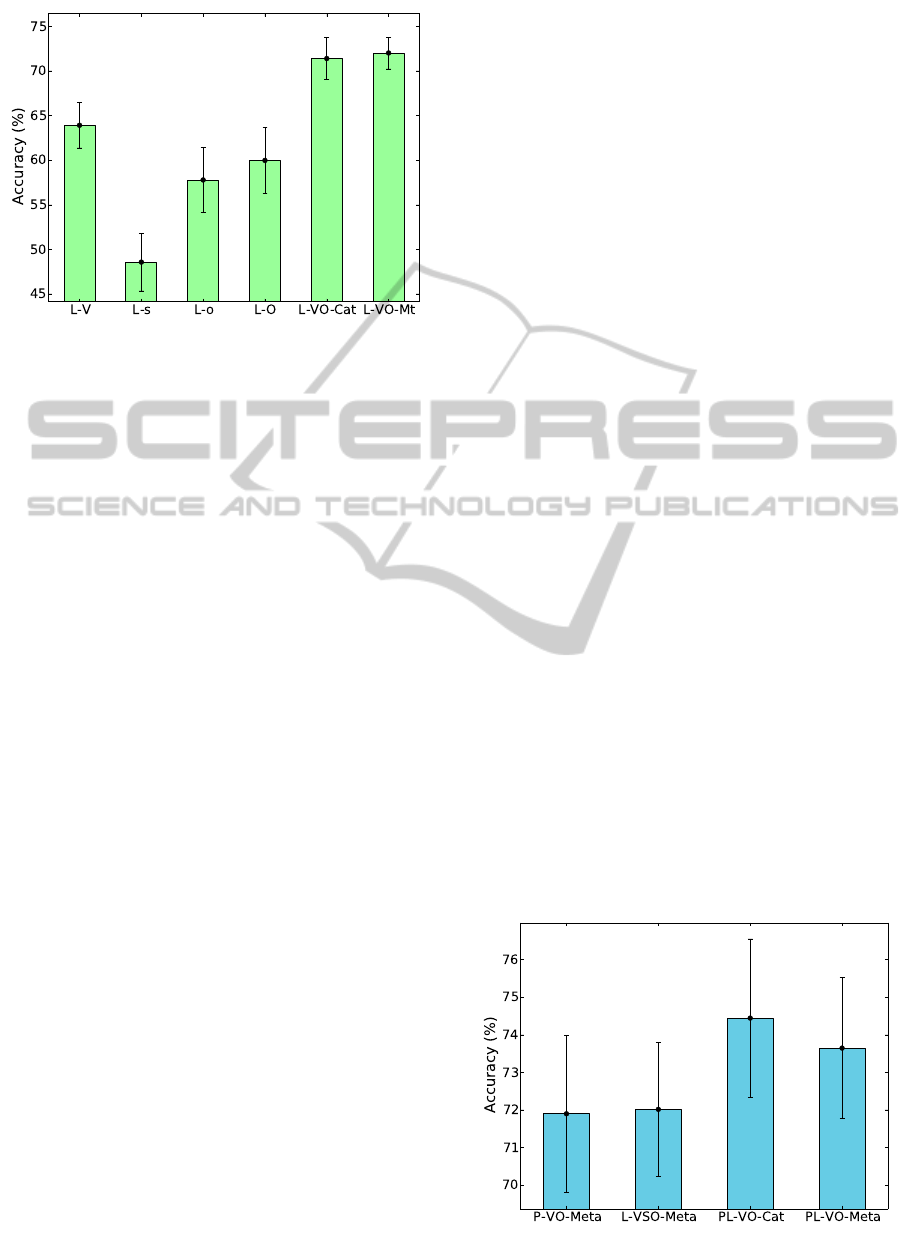
Figure 5: Using orientation with vision features for lines. L-

s and L-o respectively denote shape and orientation features

individually, and L-O concatenates both.

only one long feature vector is used; or because a

4-d orientation vector added to a 88-d vision feature

has difﬁculty making a large difference. However,

we cannot exclude the possibility that this is a con-

sequence of our choice of classiﬁer.

The next experiment was the same as the above,

but for line regions instead. Note that these evalua-

tions were done using the points which were assigned

labels from classiﬁed lines, not on the lines them-

selves (points not in lines were excluded from the

evaluation). We also tested the use of orientation (L-

o) and shape (L-s) features separately, then together

(L-O), showing that knowledge of the lines’ size and

orientation in the image, combined with the camera

orientation, is better than using the camera orienta-

tion alone. As Fig. 5 shows, the same trend as in the

points experiment is observed: orientation and shape

alone (L-O) cannot compete with vision only (L-V),

but once again combination by concatenation (L-VO-

Cat) or meta-classiﬁcation (L-VO-Meta) improve per-

formance (the latter two, like V-O, concatenate the

shape features with the orientation)

Finally, we investigated the effect of combining

point and line features. Figure 6 shows both point

and lines separately, using both types of feature (we

show the individual meta-classiﬁer versions because

they are better; points and lines appear to perform

similarly, though note that the lines were evaluated

at only a subset of points). The two methods of com-

bining entities (PL-VO-Cat and PL-VO-Meta) lead to

an improved accuracy, suggesting that combining in-

formation from multiple types of patch/region is in-

deed beneﬁcial, albeit by a smaller margin than the

above experiments. Strangely, the best performance

is achieved by PL-VO-Cat, which concatenates the

result of the less-good concatenation versions of the

individual entities, though the difference is small.

In Fig. 7 we show a confusion matrix, obtained

as the mean confusion matrix over all runs of cross-

validation, for PL-VO-Cat, the best performing vari-

ant. The diagonal is pleasingly prominent, though

there is signiﬁcant confusion between stairs and

ground (when the true class is stairs), which is some-

what unfortunate from a safety point of view. Vertical

surfaces also tend to be confused with other obstacles

and foliage, which is less of a concern. For our task,

ground identiﬁcation is perhaps the most important

criterion, which appears to be the strongest result.

6.2 Independent Data and Examples

After the cross-validation experiments, we trained

sets of (meta-)classiﬁers corresponding to different

variants of the algorithm, using the training set above

(plus copies obtained by reﬂecting across the verti-

cal image axis). We used these to evaluate perfor-

mance on the independent test set. Results are shown

in Table 1. This conﬁrms the important result of the

paper: that combining orientation information is ben-

eﬁcial, exhibiting around 10% increase in overall ac-

curacy. Adding line information did confer a further

improvement, although this was only slight. We also

show results after applying the MRF, which increased

accuracy by a few percent in each case.

We now show example results taken from the

test set, showcasing the differences between the al-

gorithms presented above. These images were chosen

to be representative examples of what the algorithms

can achieve, and where applicable, we choose the -Cat

or -Meta versions which gave the best performance in

the tests above. In all example images in the paper,

the MRF segmentation has been run, to remove noise

and give a tidier segmentation.

First, Fig. 8 shows side by side examples of the

Figure 6: Combining predictions from both points and lines.

VISAPP2015-InternationalConferenceonComputerVisionTheoryandApplications

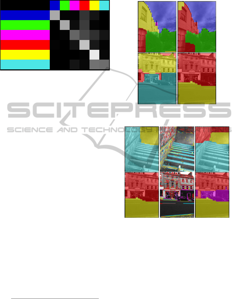
Sky

Foliage

Obstacle

Plane

Ground

Stairs

Figure 7: Confusion matrix over all runs of cross-validation,

for the best-performing algorithm PL-VO-Cat. Rows corre-

spond to the true classes, while columns represent the pre-

dicted classes. Colours correspond to those used through all

segmentation examples.

basic vision version (P-V), and the effect of adding

orientation (P-VO-Meta). In the top example, the

building fac¸ade is partly mistaken for the ground by

the visual features, whereas knowing the camera is

pointing upwards corrects this. In the bottom exam-

ple, the mis-classiﬁcation of the road as stairs is also

corrected.

In the next example (Fig. 9) we show the effect

of adding line classiﬁcations to the points-only seg-

mentation, in both cases using both visual and ori-

entation features (P-VO-Meta, PL-VO-Cat, respec-

tively). These examples show how the information

gleaned from the lines can aid segmentation, for ex-

ample by disambiguating stairs and planes, or ﬁnd-

ing non-planar objects. However, as our results below

will show, lines can sometimes be detrimental.

It is interesting to see what effect the orientation

features have, independently of the vision features,

so in Fig. 10 we show results generated using P-O

and PL-O, i.e. there are no visual features at all be-

ing used in these segmentations (image information

is being used only for line detection). Figure 10(a)

appears to be correctly segmented, but only because

this is a common and rather empty conﬁguration of

ground and walls; whereas the cars in (b) are obvi-

ously ignored. (c) is interesting since it shows that

with the camera looking down at a certain angle, stairs

Table 1: Comparison of the different algorithms on inde-

pendent test data. Using a MRF to smooth away spurious

local detections increases accuracy slightly in all cases.

Algorithm Accuracy With MRF

P-V 61.0% 64.7 %

P-VO 71.1% 73.8 %

PL-VO-Cat 71.5% 74.6 %

PL-VO-Meta 72.0% 74.3 %

Figure 8: Example results, showing segmentation using

only vision features (left) and combined with orientation

features in (right). See colour legend in Fig. 7.

Figure 9: Examples showing how adding line classiﬁca-

tions (centre) in conjunction with point features (P-VO-

Meta, left) can help improve segmentation results (PL-VO-

Cat, right).

are predicted – in this case correctly. This raises the

interesting issue that stairs are predicted here not just

because they are likely to be below the viewer, but

because the viewer is likely to look downward when

walking up stairs. In 10(d) and (e) the use of lines

has altered the segmentation, to give the impression it

is seeing the bollards and the sky (the points assume

there is sky above, but lines even at such a height are

rarely labelled as sky in the training set). In (f) the

lines themselves are shown, and it can be seen how

their orientation in the image has an effect, since the

bollards and paving stones are classiﬁed differently,

despite being at around the same image height.

UsingInertialDatatoEnhanceImageSegmentation-KnowingCameraOrientationCanImproveSegmentationofOutdoor

Scenes

(a) (b) (c) (d) (e) (f)

Figure 10: Example segmentations using only orientation information features – points only (a-c) and points with lines (d-f).

(f) shows the lines themselves, showing the effect of the lines’ orientations within the image, aiding detection of vertical posts.

More examples are shown in Fig. 11. Here, we

show the input image for clarity, plus the ground truth

segmentation which we are aiming for. The contri-

butions from vision (P-V), orientation (P-VO-Meta),

and lines (L-VO) to the ﬁnal segmentation (PL-VO-

Cat) are shown. Figures 11(a) and 11(b) again show

orientation information being used to improve clas-

siﬁcations, the latter being an interesting example

where adding lines improves segmentation even in the

presence of motion blur. Note that the different orien-

tations of the camera, such as in (c) and (d), mean that

using only position in the image as a prior would fail.

The segmentation in Fig. 11(e) also beneﬁts from

classiﬁcation of lines along the steps. Similarly in

Fig. 11(c) lines help in correctly identifying the step-

edges, but the step faces are classiﬁed as ground.

In a way this is correct, since stairs are made up

of periodic walkable regions, but this result would

be marked mostly incorrect compared to our ground

truth, which is labelled at a coarser resolution. This

echoes our comment in Section 4 about the world be-

ing ambiguous; but also that some regions may belong

to multiple classes simultaneously at different scales.

The example in 11(g) also shows orientation in-

formation being used to correctly identify the non-

ground surface; however, the addition of lines in this

case degrades the result. The ﬁnal two rows show ex-

amples where our augmented algorithms fail to pro-

vide any beneﬁt. In 11(h), the initial P-V segmenta-

tion is correct, and is unchanged by the addition of

orientation or lines (of course, if we could achieve

perfect segmentation, no amount of prior knowledge

would help). On the other hand, this illustrates why

it is so important that orientation does not impose a

hard constraint on surface identity: even when ori-

entation features are added, the grass (foliage class)

remains. In 11(i), none of the versions of the algo-

rithm are able to detect either the ground plane or the

foliage, perhaps due to the lower level of illumination.

Our implementation, comprising unoptimised

C++ code running on a Sony Vaio laptop (Intel i5,

2.40 GHz), processes one image in 1.7 seconds on

average (around 6 Hz). This is well below the cam-

era rate, but fast enough for some real-time use, when

moving at low speeds; further improvements could be

made by parallelising the code or using a GPU.

7 CONCLUSION

We have presented a way of combining information

about the real-world orientation of a camera, obtained

through inertial measurements, with more traditional

vision features, for an image segmentation algorithm.

This focused on our example application of scene seg-

mentation for locomotion in outdoor environments,

but we would expect the results to be applicable to

other types of classiﬁcation, segmentation, scene un-

derstanding and image parsing tasks where the orien-

tation of the camera is likely to effect the likelihood of

observations. We have also shown that adding orien-

tation information is beneﬁcial for line regions; and

that combining points and lines in a similar manner

can lead to some further improvement.

In our experiments it was not our intention to show

whether our method can compete with the state-of-

the art in image or scene segmentation, for example

(Gould et al., 2009) or (Domke, 2013). Rather, we

used a comparatively basic design of segmentation al-

gorithm to highlight the effect of using extra prior in-

formation, avoiding the complexity of advanced sta-

tistical techniques. An interesting avenue of further

research however to see how orientation priors can

be combined with powerful techniques such as condi-

tional random ﬁelds (Kr

ahenb

uhl and Koltun, 2011).

Other future work will look at ways to create more

accurate and detailed segmentations, and to imple-

ment this in a real-time setting. It would also be in-

teresting to combine this method with temporal in-

formation, enforcing consistency across frames; or to

combine with depth or 3D data.

VISAPP2015-InternationalConferenceonComputerVisionTheoryandApplications

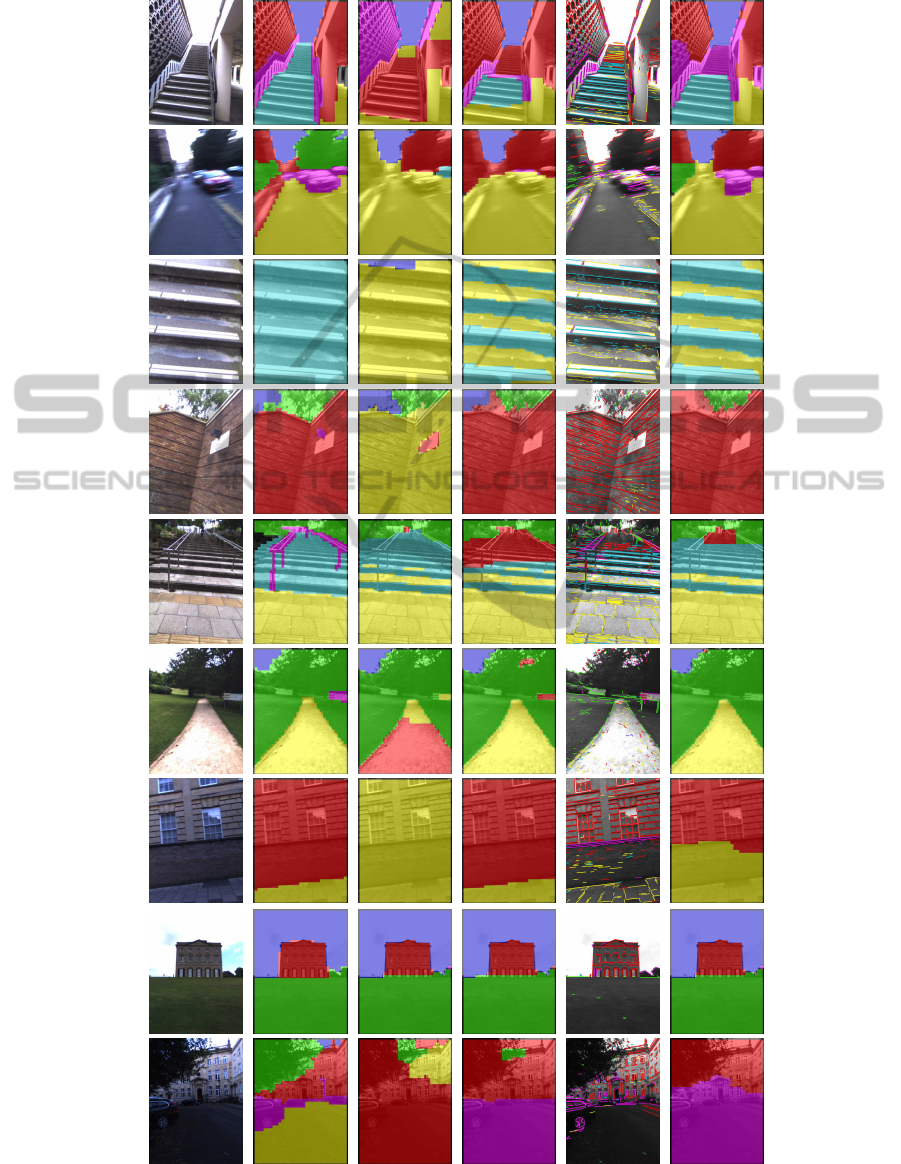
Input Ground Truth P-V P-VO-Meta L-VO-Cat PL-VO-Cat

(a)

(b)

(c)

(d)

(e)

(f)

(g)

(h)

(i)

Figure 11: Example results of the various algorithms. After the input and ground truth, we show the baseline result, of points

with only vision features (P-V), followed by adding orientation information (P-VO-Meta). Detected and vision-classiﬁed

lines are shown, before the ﬁnal result, combining everything (PL-VO-Cat).

UsingInertialDatatoEnhanceImageSegmentation-KnowingCameraOrientationCanImproveSegmentationofOutdoor

Scenes

ACKNOWLEDGEMENTS

This work was funded by the UK Engineering and

Physical Sciences Research Council (EP/J012025/1).

The authors would like to thank Austin Gregg-Smith

for advice on hardware and graphics, and Dr David

Hanwell for help with maths and text.

REFERENCES

Angelaki, D. and Cullen, K. (2008). Vestibular system: The

many facets of a multimodal sense. Annual Review of

Neuroscience, 31:125–150.

Bi, Y., Guan, J., and Bell, D. (2008). The combination of

multiple classiﬁers using an evidential reasoning ap-

proach. Artiﬁcial Intelligence, 172(15):1731–1751.

Bishop, C. (2006). Pattern Recognition and Machine

Learning. Springer.

Brock, M. and Kristensson, P. (2013). Supporting blind

navigation using depth sensing and soniﬁcation. In

Proc. Conf. Pervasive and ubiquitous computing ad-

junct publication.

Dahlkamp, H., Kaehler, A., Stavens, D., Thrun, S., and

Bradski, G. (2006). Self-supervised monocular road

detection in desert terrain. In Proc. Robotics Science

and Systems. Philadelphia.

Dalal, N. and Triggs, B. (2005). Histograms of oriented

gradients for human detection. In Proc. IEEE Conf.

Computer Vision and Pattern Recognition.

Delong, A., Osokin, A., Isack, H. N., and Boykov, Y.

(2012). Fast approximate energy minimization with

label costs. International journal of computer vision,

96(1):1–27.

Deshpande, N. and Patla, A. (2007). Visual–vestibular in-

teraction during goal directed locomotion: effects of

aging and blurring vision. Experimental brain re-

search, 176(1):43–53.

DeSouza, G. and Kak, A. (2002). Vision for mobile robot

navigation: A survey. IEEE Trans. Pattern Analysis

and Machine Intelligence, 24(2):237–267.

Domke, J. (2013). Learning graphical model parame-

ters with approximate marginal inference. IEEE

Trans. Pattern Analysis and Machine Intelligence,

35(10):2454.

Gould, S., Fulton, R., and Koller, D. (2009). Decomposing

a scene into geometric and semantically consistent re-

gions. In Proc. IEEE Int. Conf. Computer Vision.

Gupta, S., Arbel

aez, P., Girshick, R., and Malik, J.

(2014). Indoor scene understanding with rgb-d im-

ages: Bottom-up segmentation, object detection and

semantic segmentation. Int. Journal of Computer Vi-

sion, pages 1–17.

Haines, O. and Calway, A. (2012). Detecting planes and

estimating their orientation from a single image. In

Proc. British Machine Vision Conf.

Hoiem, D., Efros, A., and Hebert, M. (2007). Recovering

surface layout from an image. Int. Journal of Com-

puter Vision, 75(1):151–172.

Joshi, N., Kang, S., Zitnick, C., and Szeliski, R. (2010).

Image deblurring using inertial measurement sensors.

ACM Trans. Graphics, 29(4):30.

Kleiner, A. and Dornhege, C. (2007). Real-time localization

and elevation mapping within urban search and rescue

scenarios. Journal of Field Robotics, 24(8-9):723–

745.

ahenb

uhl, P. and Koltun, V. (2011). Efﬁcient inference in

fully connected crfs with gaussian edge potentials. In

Advances in Neural Information Processing Systems,

pages 109–117.

Kundu, A., Li, Y., Dellaert, F., Li, F., and Rehg, J. (2014).

Joint semantic segmentation and 3d reconstruction

from monocular video. In Proc. European Conf. Com-

puter Vision.

Li, S. (2009). Markov Random Field Modeling in Image

Analysis. Springer-Verlag.

Lorch, O., Albert, A., Denk, J., Gerecke, M., Cupec, R.,

Seara, J., Gerth, W., and Schmidt, G. (2002). Experi-

ments in vision-guided biped walking. In Proc. IEEE

Int. Conf. Intelligent Robots and Systems.

Maimone, M., Cheng, Y., and Matthies, L. (2007). Two

years of visual odometry on the mars exploration

rovers. Journal of Field Robotics, 24(3):169–186.

utzi, G., Weiss, S., Scaramuzza, D., and Siegwart, R.

(2011). Fusion of imu and vision for absolute scale

estimation in monocular slam. Journal of Intelligent

and Robotic Systems, 61(1-4):287–299.

Patla, A. (1997). Understanding the roles of vision in

the control of human locomotion. Gait & Posture,

5(1):54–69.

Pini

es, P., Lupton, T., Sukkarieh, S., and Tard

os, J. (2007).

Inertial aiding of inverse depth slam using a monoc-

ular camera. In Proc. IEEE Int. Conf. Robotics and

Automation.

Sadhukhan, D., Moore, C., and E., C. (2004). Terrain esti-

mation using internal sensors. In Proc. Int. Conf. on

Robotics and Applications.

Sturgess, P., Alahari, K., Ladicky, L., and Torr, P. (2009).

Combining appearance and structure from motion fea-

tures for road scene understanding. In Proc. British

Machine Vision Conf.

Tapu, R., Mocanu, B., and Zaharia, T. (2013). A computer

vision system that ensure the autonomous navigation

of blind people. In Proc. Conf. E-Health and Bioengi-

neering.

Virre, E. (1996). Virtual reality and the vestibular appara-

tus. Engineering in Medicine and Biology Magazine,

15(2):41–43.

Von Gioi, R., Jakubowicz, J., Morel, J., and Randall, G.

(2010). Lsd: A fast line segment detector with a false

detection control. IEEE Trans. Pattern Analysis and

Machine Intelligence, 32(4):722–732.

VISAPP2015-InternationalConferenceonComputerVisionTheoryandApplications