Finding Resilient Solutions for Dynamic Multi-Objective Constraint
Optimization Problems
Maxime Clement
1
, Tenda Okimoto
2,3
, Nicolas Schwind
3,4
and Katsumi Inoue
4,1
1
Department of Informatics, The Graduate University for Advanced Studies, Tokyo, Japan
2
Faculty of Maritime Sciences, Kobe University, Kobe, Japan
3
Transdisciplinary Research Integration Center, Tokyo, Japan
4
National Institute of Informatics, Tokyo, Japan
Keywords:
Systems Resilience, Dynamic Multi-Objective COP, Resistance, Functionality, Reactive Approach.
Abstract:
Systems Resilience is a large-scale multi-disciplinary research that aims to identify general principles under-
lying the resilience of real world complex systems. Many conceptual frameworks have been proposed and
discussed in the literature since Holling’s seminal paper (1973). Schwind et al. (2013) recently adopted a
computational point of view of Systems Resilience, and modeled a resilient system as a dynamic constraint
optimization problem. However, many real world optimization problems involve multiple criteria that should
be considered separately and optimized simultaneously. Also, it is important to provide an algorithm that can
evaluate the resilience of a dynamic system. In this paper, a framework for Dynamic Multi-Objective Con-
straint Optimization Problem (DMO-COP) is introduced and two solution criteria for solving this problem are
provided, namely resistance and functionality, which are properties of interest underlying the resilience for
DMO-COPs. Also, as an initial step toward developing an efficient algorithm for finding resilient solutions
of a DMO-COP, an algorithm called Algorithm for Systems Resilience (ASR), which computes every resistant
and functional solution for DMO-COPs, is presented and evaluated with different types of dynamical changes.
1 INTRODUCTION
Many researchers of different fields have recognized
the importance of a new research discipline con-
cerning the resilience of real world complex sys-
tems (Holling, 1973; Bruneau, 2003; Walker et al.,
2004; Longstaff et al., 2010). The concept of re-
silience has appeared in various disciplines, e.g., en-
vironmental science, materials science and sociology.
The goal of resilience research is to provide a set
of general principles for building resilient systems in
various domains, such that the systems are resistant
from large-scale perturbations caused by unexpected
events and changes, and keep their functionality in the
long run. Holling (1973) first introduced the concept
of resilience as an important characteristic of a well-
behaved ecological system, and defined it as the ca-
pacity of an ecosystem to respond to a perturbation
or disturbance by resisting damage. He adopted a
verbal, qualitative definition of ecological resilience,
rather than a mathematical, quantitative one. “Re-
silience determines the persistence of relationships
within a system and is a measure of the ability of these
systems to absorb changes of state variables, driving
variables, and parameters, and still persist.” (Holling,
1973, page 17). Schwind et al.(2013) adopted a com-
putational point of view of Systems Resilience, and
modeled a resilient system as a dynamic constraint-
based model (called SR-model), i.e., dynamic con-
straint optimization problem. They captured the no-
tion of resilience using several factors, e.g., resis-
tance, recoverability, functionality and stabilizability.
Capturing and evaluating the resilience of realistic
dynamic systems often requires to (i) consider several
objectives to optimize simultaneously from the point
of view of the resilience factors, and (ii) develop an
algorithm for solving this problem. This is the main
purpose of this paper.
A Multi-Objective Constraint Optimization Prob-
lem (MO-COP) (Junker, 2006; Marinescu, 2010; Rol-
lon and Larrosa, 2006) is the extension of a mono-
objective COP (Dechter, 2003; Schiex et al., 1995).
Solving a COP consists in finding an assignment of
values to variables so that the sum of the result-
ing costs is minimized. A wide variety of Artifi-
cial Intelligence problems can be formalized as COPs,
509
Clement M., Okimoto T., Schwind N. and Inoue K..
Finding Resilient Solutions for Dynamic Multi-Objective Constraint Optimization Problems.
DOI: 10.5220/0005276305090516
In Proceedings of the International Conference on Agents and Artificial Intelligence (ICAART-2015), pages 509-516
ISBN: 978-989-758-074-1
Copyright
c
 2015 SCITEPRESS (Science and Technology Publications, Lda.)

e.g., resource allocation problem (Cabon et al., 1999),
scheduling (Verfaillie et al., 1996) and combinatorial
auctions (Sandholm, 1999). In an MO-COP, gen-
erally, since trade-offs exist among objectives, there
does not exist an ideal assignment, which minimizes
all objectives simultaneously. Thus, the “optimal” so-
lution of an MO-COP is characterized using the con-
cept of Pareto optimality. An assignment is a Pareto
optimal solution if there does not exist another assign-
ment that weakly improves all of the objectives. Solv-
ing an MO-COP is to find the Pareto front which is a
set of cost vectors obtained by all Pareto optimal so-
lutions. Most works on MO-COPs consist in devel-
oping efficient algorithms for solving static problems
(Marinescu, 2010; Perny and Spanjaard, 2008; Rollon
and Larrosa, 2006; Rollon and Larrosa, 2007). How-
ever, due to the dynamic nature of our environment,
many real-world problems change through time.
In this paper, a framework for Dynamic Multi-
Objective Constraint Optimization Problem (DMO-
COP) is introduced, which is the extension of MO-
COP and dynamic COP. Also, two solution criteria for
solving this problem are provided, namely resistance
and functionality, which are properties of interest un-
derlying the resilience for DMO-COPs. Our model
is defined by a sequence of MO-COPs representing
the changes within a system that is subject to exter-
nal fluctuations. The resistance is the ability to main-
tain some underlining costs under a certain threshold,
such that the system satisfies certain hard constraint
and does not suffer from irreversible damages. The
functionality is the ability to maintain a guaranteed
global quality for the configuration trajectory in a se-
quence. These two properties are central in the char-
acterization of “robust” solution trajectories, which
keep a certain quality level and “absorb” external fluc-
tuations without suffering degradation. Indeed, these
notions are consistent with the initial formulation of
resilience from (Holling, 1973). An algorithm called
Algorithm for Systems Resilience (ASR) for solving a
DMO-COP is presented. This algorithm is based on
the branch and bound search, which is widely used
for COP and MO-COP algorithms, and it finds all re-
sistant and functional solutions for DMO-COP. In the
experiments, the performances of ASR are evaluated
with different types of dynamical changes.
We believe that the computational design of re-
silient systems is a promising area of research, rele-
vant for many applications like sensor networks. A
sensor network is a resource allocation problem that
can be formalized as a COP (Cabon et al., 1999).
For example, consider a sensor network in a territory,
where each sensor can sense a certain area in this ter-
ritory. When we consider this problem with multiple
x
1
x
2
cost
a a 5
a b 7
b a 10
b b 12
x
2
x
3
cost
a a 0
a b 2
b a 0
b b 2
x
1
x
3
cost
a a 1
a b 1
b a 0
b b 3
Figure 1: Example of mono-objective COP.
criteria, e.g., data management, quality of observation
data and electrical consumption, it can be formalized
as an MO-COP (Okimoto et al., 2014). Additionally,
when we consider some accidents, e.g., sensing er-
ror, breakdown and electricity failure, it can be repre-
sented by the dynamical change of constraint costs.
The rest of the paper is organized as follows. In
the next section, the formalizations of COP and MO-
COP are briefly introduced. The following section
presents our framework for DMO-COP and the com-
putation of resistant and functionalsolutions. Also, an
algorithm called ASR is presented. Afterwards, some
empirical results are provided. Just before the con-
cluding section, some related works are discussed.
2 PRELIMINARIES
2.1 COP
A Constraint Optimization Problem (COP) (Dechter,
2003; Schiex et al., 1995) consists in finding an as-
signment of values to variables so that the sum of
the resulting costs is minimized. A COP is de-
fined by a set of variables X, a set of constraint re-
lations C, and a set of cost functions F. A vari-
able x
i
takes its value from a finite, discrete do-
main D
i
. A constraint relation (i, j) means there ex-
ists a constraint relation between x
i
and x
j
.
1
For
x
i
and x
j
, which have a constraint relation, the cost
for an assignment {(x
i
,d
i
),(x
j
,d
j
)} is defined by a
cost function f
i, j
: D
i
× D
j
→ R
+
. For a value as-
signment to all variables A, let us denote R(A) =
∑
(i, j)∈C,{(x
i
,d
i
),(x
j
,d
j
)}⊆A
f
i, j
(d
i
,d
j
), where d
i
∈ D
i
and
d
j
∈ D
j
. Then, an optimal assignment A
∗
is given
1
In this paper, we assume that all constraints are binary
for simplicity like many existing COP papers. Relaxing this
assumption to general cases is relatively straightforward.
ICAART2015-InternationalConferenceonAgentsandArtificialIntelligence
510

as argmin
A
R(A), i.e., A
∗
is an assignment that mini-
mizes the sum of the value of all cost functions, and an
optimal value is given by R(A
∗
). A COP can be rep-
resented using a constraint graph, in which nodes cor-
respond to variables and edges represent constraints.
Example 1 (COP). Figure 1 shows a mono-objective
COP with three variables x
1
,x
2
and x
3
. Each vari-
able takes its value assignment from a discrete do-
main {a,b}. The figure showsthree cost tables among
three variables. The optimal solution of this problem
is {(x
1
,a),(x
2
,a),(x
3
,a)}, and the optimal value is 6.
2.2 MO-COP
A Multi-Objective Constraint Optimization Problem
(MO-COP) (Junker, 2006; Marinescu, 2010; Rol-
lon and Larrosa, 2006) is defined by a set of vari-
ables X = {x
1
,x
2
,...,x
n
}, multi-objective constraints
C = {C
1
,C
2
,...,C
m
}, i.e., a set of sets of con-
straint relations, and multi-objective functions F =
{F
1
,F
2
,...,F
m
}, i.e., a set of sets of objective func-
tions. For an objective h (1 ≤ h ≤ m), variables
x
i
and x
j
, which have a constraint relation, the cost
for an assignment {(x
i
,d
i
),(x
j
,d
j
)} is defined by a
cost function f
h
i, j
: D
i
× D
j
→ R
+
. For an objective
h and a value assignment to all variables A, let us
denote R
h
(A) =
∑
(i, j)∈C
h
,{(x
i
,d
i
),(x
j
,d
j
)}⊆A
f
h
i, j
(d
i
,d
j
).
Then, the sum of the values of all cost functions
for m objectives is defined by a cost vector, denoted
R(A) = (R
1
(A),R
2
(A),. ..,R
m
(A)). To find an assign-
ment that minimizes all m objective functions simul-
taneously is ideal. However, in general, since trade-
offs exist among objectives, there does not exist such
an ideal assignment. Therefore, the “optimal” solu-
tion of an MO-COP is characterized by using the con-
cept of Pareto optimality. An assignment is a Pareto
optimal solution if there does not exist another assign-
ment that weakly improves all of the objectives. Solv-
ing an MO-COP is to find the Pareto front which is a
set of cost vectors obtained by all Pareto optimal so-
lutions. In an MO-COP, the number of Pareto optimal
solutions is often exponential in the number of vari-
ables, i.e., every possible assignment can be a Pareto
optimal solution in the worst case. This problem can
be also represented as a constraint graph.
Definition 1 (Dominance). For an MO-COP and two
cost vectors R(A) and R(A
′
), we say that R(A) domi-
nates R(A
′
), denoted by R(A) ≺ R(A
′
), iff R(A) is par-
tially less than R(A
′
), i.e., it holds (i) R
h
(A) ≤ R
h
(A
′
)
for all objectives h, and (ii) there exists at least one
objective h
′
, such that R
h
′
(A) < R
h
′
(A
′
).
Definition 2 (Pareto optimal solution). For an MO-
COP, an assignment A is said to be the Pareto optimal
Table 1: Example of bi-objective COP.
x
1
x
2
cost x
2
x
3
cost x
1
x
3
cost
a a (5,2) a a (0,1) a a (1,0)
a b (7,1) a b (2,1) a b (1,0)
b a (10,3) b a (0,2) b a (0,1)
b b (12,0) b b (2,0) b b (3,2)
solution, iff there does not exist another assignment
A
′
, such that R(A
′
) ≺ R(A).
Definition 3 (Pareto Front). Given an MO-COP, the
Pareto front is the set of cost vectors obtained by the
set of Pareto optimal solutions.
Example 2 (MO-COP). Table 1 shows a bi-objective
COP, which is an extension of the COP in Figure 1.
Each variable takes its value from a discrete domain
{a,b}. The Pareto optimal solutions of this prob-
lem are {{(x
1
,a), (x
2
,a), (x
3
,a)}, {(x
1
,a), (x
2
,b),
(x
3
,b)}}, and the Pareto front is {(6,3), (10, 1)}.
3 DYNAMIC MO-COP
In this section, a framework for Dynamic Multi-
Objective Constraint Optimization Problem (DMO-
COP) is introduced and two solution criteria for solv-
ing this problem are provided: resistance and func-
tionality. Furthermore, an algorithm called Algorithm
for Systems Resilience (ASR) is presented.
3.1 Model
A framework of DMO-COP is defined by a sequence
of MO-COPs as follows
2
:
DMO-COP = hMO-COP
0
,MO-COP
1
,. .. ,MO-COP
k
i,
where each index i (0 ≤ i ≤ k) represents a time step.
Solving a DMO-COP is finding the following se-
quence of Pareto front, denoted PF, where each PF
i
(0 ≤ i ≤ k) represents the Pareto front of MO-COP
i
.
PF = hPF
0
,PF
1
,...,PF
k
i.
Our focus is laid on a reactive approach, i.e., each
problem MO-COP
i
in a DMO-COP can only be
known at time step i (0 ≤ i ≤ k), and we have no
information about the problems for any time step
j where j > i. For dynamic problems, there exist
two approaches, namely proactive and reactive. In a
proactive approach, all problems in a DMO-COP are
known in advance. Since we know all changes among
problems, one possible goal of this approach is to find
2
Similar formalization, i.e., dynamic problem as a se-
quence of static problems, is provided in many previous
works such as (Okimoto et al., 2014; Yeoh et al., 2011).
FindingResilientSolutionsforDynamicMulti-ObjectiveConstraintOptimizationProblems
511

Table 2: Cost table of MO-COP
1
.
x
1
x
2
cost x
2
x
3
cost x
1
x
3
cost
a a (5,2) a a (0,1) a a (1,0)
a b (7,1) a b (2,1) a b (5,5)
b a (10,3) b a (0,2) b a (0,1)
b b (12,0) b b (2,0) b b (1,1)
Table 3: Cost table of MO-COP
2
.
x
1
x
2
cost x
2
x
3
cost x
1
x
3
cost
a a (5,2) a a (3,3) a a (4,4)
a b (7,1) a b (2,1) a b (5,5)
b a (2,2) b a (0,2) b a (0,1)
b b (3,0) b b (2,0) b b (1,1)
an optimal solution for a DMO-COP. On the other
hand, in a reactive approach, since the new problem
typically arises after solving the previous problem, it
requires to solve each problem in a DMO-COP one
by one. Thus, we need to find a sequence of Pareto
front. In the following, the change of the constraint
costs among problems in a DMO-COP is studied.
3
Example 3. Consider a DMO-COP = hMO-COP
0
,
MO-COP
1
, MO-COP
2
i. We use the same exam-
ple represented in Example 2 and use it as the ini-
tial problem of this DMO-COP. The Pareto optimal
solutions of MO-COP
0
are {(x
1
,a), (x
2
,a), (x
3
,a)}
and {(x
1
,a), (x
2
,b), (x
3
,b)}, and the Pareto front is
{(6,3), (10, 1)} (see. Example 2). Table 2 shows
the cost table of MO-COP
1
. In Table 2, two con-
straints written in boldface are dynamically changed
from the initial problem MO-COP
0
, i.e., the cost
vector of {(x
1
,a), (x
3
,b)} and {(x
1
,b), (x
3
,b)} are
changed from (1,0) to (5,5) and from (3, 2) to
(1,1). The Pareto optimal solutions of MO-COP
1
are
{(x
1
,a), (x
2
,a), (x
3
,a)} and {(x
1
,b), (x
2
,b),(x
3
,b)},
and the Pareto front is {(6,3), (15,1)}. Table 3
represents the cost vector of MO-COP
2
. In Ta-
ble 3, four constraints written in boldface are addi-
tionally changed from MO-COP
1
i.e., (2,2), (3,0),
(3,3), and (4,4). The Pareto optimal solutions of
MO-COP
2
are {(x
1
,b), (x
2
,b), (x
3
,a)} and {(x
1
,b),
(x
2
,b),(x
3
,b)}, and the Pareto front is {(3,3), (6, 1)}.
Thus, the solution of this DMO-COP is PF =
{{(6,3),(10,1)},{(6,3),(15,1)},{(3,3),(6,1)}}.
Now, two solution criteria for DMO-COPs are
provided, namely, resistance and functionality. A se-
quence of assignments A = hA
0
,A
1
,...,A
j
i is called
an assignment trajectory, where A
i
is an assignment
of MO-COP
i
(0 ≤ i ≤ j). Let m be the number of
3
Other changes, e.g., the number of variables, objectives
and domain size, can be also considered. In this paper, the
focus is laid on the dynamical change of constraint costs
among problems. Similar assumption is also introduced in
previous works (Okimoto et al., 2014; Yeoh et al., 2011).
objectives and R
h
(A
i
) be the cost for objective h ob-
tained by assignment A
i
(1 ≤ h ≤ m), and l, q be con-
stant vectors.
Definition 4 (Resistance). For an assignment trajec-
tory A and a constant vector l = (l
1
,l
2
,...,l
m
), A is
said to be l-resistant, iff for all h (1 ≤ h ≤ m),
R
h
(A
i
) ≤ l
h
, (0 ≤ i ≤ |A| − 1).
Definition 5 (Functionality). For an assignment tra-
jectory A and a constant vector q = (q
1
,q
2
,...,q
m
), A
is said to be q-functional, iff for all h (1 ≤ h ≤ m) and
for each j ∈ {0,.. .,|A| − 1},
∑
j
i=0
R
h
(A
i
)
j + 1
≤ q
h
.
Resistance is the ability to maintain some under-
lining costs under a certain threshold, such that the
system satisfies certain hard constraint and does not
suffer from irreversible damages, i.e., the ability for a
system to stay essentially unchanged despite the pres-
ence of disturbances. Functionality is the ability to
maintain a guaranteed global quality for the assign-
ment trajectory. While resistance requires to main-
tain a certain quality level at each problem in a DMO-
COP, functionality requires to maintain this level in
average, when looking over a certain horizon of time.
Thus, functionality evaluates an assignment trajectory
globally. The followings are two examples for them.
We use the same example as in Example 3.
Example 4 (Resistance). The Pareto optimal solu-
tions of the DMO-COP is {(x
1
,a), (x
2
,a), (x
3
,a)}
and {(x
1
,a), (x
2
,b), (x
3
,b)} for MO-COP
0
, {(x
1
,a),
(x
2
,a), (x
3
,a)} and {(x
1
,b), (x
2
,b), (x
3
,b)} for MO-
COP
1
, and {(x
1
,b), (x
2
,b), (x
3
,a)} and {(x
1
,b),
(x
2
,b), (x
3
,b)} for MO-COP
2
. The correspond-
ing Pareto front is PF
0
= {(6,3),(10,1)}, PF
1
=
{(6,3),(15,1)}, and PF
2
= {(3,3),(6, 1)}, respec-
tively. Let l = (8,4) be a constant vector.
The assignment trajectory A = hA
0
,A
1
,A
2
i with
A
0
= {(x
1
,a),(x
2
,a),(x
3
,a)}, A
1
= {(x
1
,a), (x
2
,a),
(x
3
,a)}, and A
2
= {(x
1
,b), (x
2
,b), (x
3
,a)} is l-
resistant, since R
1
(A
0
) = 6 < l
1
(= 8), R
2
(A
0
) =
3 < l
2
(= 4), R
1
(A
1
) = 6 < l
1
, R
2
(A
1
) = 3 < l
2
,
and R
1
(A
2
) = 3 < l
1
,R
2
(A
2
) = 3 < l
2
. Similarly,
A
′
= hA
0
,A
1
,A
′
2
i is also l-resistant, where A
0
and A
1
are same as in A and A
′
2
= {(x
1
,b), (x
2
,b), (x
3
,b)}.
Example 5 (Functionality). Let q = (5,4) be a con-
stant vector. The assignment trajectory A = hA
0
, A
1
,
A
2
i with A
0
= {(x
1
,a), (x
2
,a), (x
3
,a)}, A
1
= {(x
1
,a),
(x
2
,a), (x
3
,a)}, and A
2
= {(x
1
,b), (x
2
,b), (x
3
,a)}
is q-functional, since (6 + 6 + 3)/3 = 5 ≤ q
1
(= 5)
ICAART2015-InternationalConferenceonAgentsandArtificialIntelligence
512

and (3 + 3 + 3)/3 = 3 < q
2
(= 4). However, for
A
′
= hA
0
,A
1
,A
′
2
i where A
0
and A
1
are same as in
A and A
′
2
= {(x
1
,b), (x
2
,b), (x
3
,b)}, A
′
is not q-
functional, since (6+ 6 + 6)/3= 6 > q
1
(= 5).
3.2 Algorithm
An algorithm, Algorithm for Systems Resilience
(ASR), for solving a DMO-COP is presented. This
algorithm is based on the branch-and-bound search,
which is widely used for COP and MO-COP al-
gorithms, and it finds all resistant and functional
solutions for DMO-COPs. Algorithm 1 shows the
pseudo-code of ASR. The input is a DMO-COP that
is a sequence of MO-COPs and constant vectors l
and q. ASR outputs a set of sequences (all l-resistant
and q-functional solutions). For each MO-COP
i
(0 ≤ i ≤ k) in the sequence, ASR computes a set
of all l-resistant solutions denoted RS
l
i
by ASR
res
(line 6). ASR uses the ⊗-operator and combines
the set of sequences RS and the cost vectors of
RS
l
i
obtained by ASR
res
(line 10). For example,
after the combination of RS = {(6,3),(10,1)}
and RS
l
1
= {(6,3),(15,1)}, i.e., RS ⊗ RS
l
1
,
there exist four sequences {{(6,3)},{(6,3)}},
{{(6,3)},{(15,1)}}, {{(10, 1)},{(6,3)}} and
{{(10, 1)},{(15,1)}}. For the initial problem, i.e.,
MO-COP
0
, RS is equal to RS
l
0
when RS
l
0
6=
/
0. Next,
ASR checks the q-functionality of each sequence of
RS (line 11). Finally, it provides a set of all l-resistant
and q-functional solutions. Otherwise, it outputs the
empty set (checked in line 7-9 and line 12-14). In
case l and q are large enough (i.e., no restriction), all
Pareto optimal solutions may become l-resistant and
Algorithm 1: ASR.
1: INPUT : DMO-COP = hMO-COP
0
, MO-COP
1
, ...,
MO-COP
k
i and two constant vectors l = (l
1
,l
2
,...,l
m
), q =
(q
1
,q
2
,...,q
m
)
2: OUTPUT : RS // set of sequences (all l-resistant and q-
functional solutions)
3: RS ←
/
0
4: l, q ← constant vectors
5: for each MO-COP
i
(i = 0,...,k) do
6: RS
l
i
← ASR
res
(MO-COP
i
,l) // find all l-resistant solutions
7: if RS
l
i
=
/
0 then
8: return RS ←
/
0
9: end if
10: RS ← RS ⊗ RS
l
i
// combine the current solution with pre-
vious solutions
11: RS
q
← ASR
fun
(RS,q) // filter RS with q-functionality
12: if RS
q
=
/
0 then
13: return RS ←
/
0
14: end if
15: RS ← RS
q
16: end for
17: return RS
Algorithm 2: ASR
res
.
1: INPUT : MO-COP
i
and l
2: OUTPUT : RS
l
i
// a set of l-resistant solutions of MO-COP
i
3: Root : // the root of MO-COP
i
4: AS ←
/
0 // an assignment of variables
5: Cost ← null vector // cost vector obtained by AS
6: RS
l
i
←
/
0 // a set of pairs <cost vector, set of assignments>
// Launch solving from the root
7: RS
l
i
← first.solve(AS,Cost, RS
l
i
,l)
8: return RS
l
i
Algorithm 3: solve(AS,Cost,RS
l
i
,l).
1: INPUT : < AS,Cost,RS
l
i
,l >
2: OUTPUT : RS
l
i
3: for each value v
1
of the variable domain do
4: AS ← v
1
5: local
cost ← null vector
// step 3.1: Compute local cost of the choice
6: for each constraint with an ancestor a do
7: v
2
← value of a in AS
8: local
cost ← local cost + cost(v
1
,v
2
)
9: end for
10: new
cost ← Cost + local cost
// step 3.2: Bound checking
11: dominated ← false
12: for each objective h (1 ≤ h ≤ m) do
13: if r
h
> l
h
,r
h
∈ new
cost then
14: AS ← (AS\ v
1
)
15: dominated ← true
16: end if
17: end for
18: if new
cost is dominated by RS
l
i
then
19: AS ← (AS\ v
1
)
20: dominated ← true
21: end if
22: if dominated then
23: continue
24: end if
// step 3.3.1: New Pareto optimal solution
25: if AS is complete then
26: E ← all elements of RS
l
i
dominated by new
cost
27: RS
l
i
← RS
l
i
\ E
28: RS
l
i
← RS
l
i
∪ {(new
cost,AS)}
29: continue
30: end if
// step 3.3.2: Continue solving
31: RS
l
i
← next.solve(AS,Cost,RS
l
i
,l)
32: AS ← (AS\ v
1
)
33: end for
34: return RS
l
i
q-functional solutions in the worst case, and the size
of RS finally becomes |RS
0
| × |RS
1
| × ... × |RS
k
|.
Let us describe ASR
res
. It finds all Pareto opti-
mal solutions of each problem in a sequence, which
are bounded by the parameter l. The pseudo-code of
ASR
res
is given in Algorithm 2 and 3. We assume that
a variable ordering, i.e., pseudo-tree (Schiex et al.,
1995), is given. The input is an MO-COP
i
(0 ≤ i ≤ k)
and a constant vector l, and the output is the entire set
of l-resistant solutions (lines 1 and 2 in Algorithm 2).
ASR
res
starts with an empty set of l-resistant solutions
and a null cost vector, and solves the first variable ac-
cording to the variable ordering (lines 3-7). It chooses
FindingResilientSolutionsforDynamicMulti-ObjectiveConstraintOptimizationProblems
513

Algorithm 4: ASR
fun
.
1: INPUT : RS,q
2: OUTPUT : RS
q
// set of the filtered sequences
3: RS
q
←
/
0
4: for each sequence S
j
∈ RS (0 ≤ j ≤ |RS| − 1) do
5: for each h (1 ≤ h ≤ m) do
6: if
∑
|S
j
|−1
i=0
s
h
i, j
|S
j
|
> q
h
// s
i, j
∈ S
j
then
7: return RS
q
=
/
0
8: end if
9: end for
10: RS
q
← S
j
11: end for
12: return RS
q
a value for the variable and updates the cost vector
according to the cost tables (step 3.1 in Algorithm 3).
At this moment the obtained cost vector has to ensure
the following two properties: (i) r
h
(the cost for ob-
jective h) is bounded by the constant vector l and (ii)
the cost vector is not dominated by another cost vec-
tor (i.e., current l-resistant solutions) in RS
l
i
. If one of
the two properties is violated, ASR
res
branches on the
next value of the variable. When its domain is com-
pletely explored, the search branches to the previous
variable and continues the solving (step 3.2 in Algo-
rithm 3). When all assignments are formed, i.e., no
variable left to be assigned, a new solution is added to
RS
l
i
. All previous dominated solutions are removed
from RS
l
i
and the search continues with the next val-
ues of the variable (step 3.3.1 in Algorithm 3). In
case r
h
fulfills the two properties, it continues the
solving with the next variable according to the vari-
able ordering (step 3.3.2). The search stops when the
whole search space has been covered by the branch-
and-bound search. ASR
res
finally outputs the set of l-
resistant solutions (which are not dominated by other
solutions)
4
.
Let us describe ASR
fun
. Algorithm 4 shows the
pseudo-code of it. The input is a set of sequences
obtained by ASR
res
and a constant parameter q, and
output is a set of l-resistant and q-functional solu-
tions RS
q
(lines 4-11). For each sequence S
j
of RS, it
checks the q-functionality by using the equation given
in Definition 5 (lines 5-9). ASR is a complete al-
gorithm, i.e., it provides a set of all l-resistant and
q-functional solutions if there exists. Otherwise, it
outputs the empty set (lines 7-9 and 12-14 in Algo-
rithm 1).
4
ASR
res
checks the dominance among the solutions (in
lines 18, 22 and 26 in Algorithm 3) and provides the set of
Pareto optimal solutions bounded by the parameter l.
4 SOME EXPERIMENTAL
RESULTS
In this section, the performances of ASR are evalu-
ated with different types of dynamical changes. In
the experiments, we generate DMO-COPs that con-
tain three MO-COPs as in Example 3. All the tests
are made with 20 variables, the domain size of each
variable is 2, the number of objectives is 2, and the
cost of each constraint is a random value between
0 and 100. In DMO-COPs, we change a fixed pro-
portion of constraint costs (called the change ratio) at
each dynamic step. For the initial problem, we choose
the constraint costs from [0:100]. Then, we create
the next problem by changing the proportion of con-
straints costs defined by the change ratio. For exam-
ple, in case the change ratio is 5%, we choose 5%
of all constraints in the current problem and change
their constraint costs by selecting the new costs from
the range [100:200], but do not change the remaining
constraint costs. Each data point in a graph represents
the average of 50 problem instances.
Figure 2 and 3 show the average number of solu-
tions and its runtime obtained by ASR. The l-ratio is
provided by l/(cost
max
× #constraints), where cost
max
is the maximal cost value (i.e., 200). We vary the the
change ratio from 0.05 to 0.5 and from 0.3 to 1.0 for
l-ratio. In this experiment, we set the constant vec-
tor to q = (q
max
,q
max
), where q
max
= 3 × (cost
max
×
0.3
0.4
0.5
0.6
0.7
0.8
0.9
1
0.05
0.1
0.15
0.2
0.25
0.3
0.35
0.4
0.45
0.5
0
4000
8000
12000
16000
solutions
l-ratio
change ratio
solutions
0
2000
4000
6000
8000
10000
12000
14000
16000
18000
20000
Figure 2: Number of solutions.
0.3
0.4
0.5
0.6
0.7
0.8
0.9
1
0.05
0.1
0.15
0.2
0.25
0.3
0.35
0.4
0.45
0.5
0
5
10
15
20
25
t(s)
l-ratio
change ratio
t(s)
0
5
10
15
20
25
Figure 3: Runtime.
ICAART2015-InternationalConferenceonAgentsandArtificialIntelligence
514

10
100
1000
10000
100000
0.05 0.15 0.25 0.35 0.45 0.5
#sols0
#sols1
#sols2
(a) q-ratio is 0.2.
10
100
1000
10000
100000
0.05 0.15 0.25 0.35 0.45 0.5
#sols0
#sols1
#sols2
(b) q-ratio is 0.4.
10
100
1000
10000
100000
0.05 0.15 0.25 0.35 0.45 0.5
#sols0
#sols1
#sols2
(c) q-ratio is 0.6.
10
100
1000
10000
100000
0.05 0.15 0.25 0.35 0.45 0.5
#sols0
#sols1
#sols2
(d) q-ratio is 0.8.
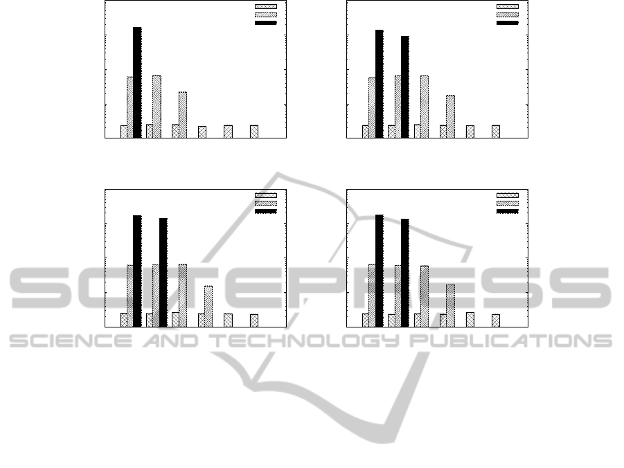
Figure 4: The average number of resistant and functional solutions of each problem in DMO-COPs.
#constraints) which is large enough, so that all l-
resistant solutions become q-functional. In figure 2,
we can observe that only small change ratio (i.e., from
0.05 to 0.15) for the l-ratio from 0.5 to 1.0 allows
us to find resistant (and also functional) solutions for
DMO-COPs. On the other hand, in case the l-ratio is
small and the change ratio is large, ASR cannot find
any solutions. In figure 3, we observed that the aver-
age runtime increases where the number of resistant
(and also functional) solutions becomes large.
Figure 4 shows the results for the average num-
ber of obtained resistant and functional solutions of
each problem in DMO-COP, i.e., MO-COP
0
, MO-
COP
1
and MO-COP
2
, for varying the q-ratio. In this
experiment, we set l-ratio to 0.8. The #sols0 repre-
sents the number of obtained resistant and functional
solutions in MO-COP
0
, #sols1 is for MO-COP
1
, and
#sols2 shows that for MO-COP
2
. The x axis shows
the change ratio and the y axis is the number of so-
lutions obtained by ASR. For any q-ratio, we find
solutions for the initial problem (i.e., MO-COP
0
) in
DMO-COPs. It is the problem where Pareto opti-
mal solutions have the lowest cost vectors. Once this
problem changes (with regard to the change ratio), the
average cost vector increases and the functionality be-
comes harder to obtain. For small changes where the
change ratio is 0.05, even a low q-ratio (q = 0.2) al-
lows to find resistant and functional solutions (Fig-
ure 4(a)). However, for more drastic changes, e.g., the
change ration is 0.15, we need a higher q-ratio in or-
der to find solutions after the third problem. We then
reach a point where the change ratios are too severe
(i.e., 0.25-0.5) to find solutions for the third problem.
We can increase the q-ratio but we cannot find resis-
tant and functional solutions (Figure 4(b)- 4(d)).
In summary, these experimental results reveal
that the performance of ASR is highly influenced by
change ratio. ASR can obtain the resistant and func-
tional solutions of a DMO-COP, when the dynamical
changes are small (i.e. the change ratio is from 0.05
to 0.15). Otherwise, ASR outputs empty set quickly.
5 RELATED WORKS
Various algorithms have been developed for MO-
COPs (Marinescu, 2010; Perny and Spanjaard, 2008;
Rollon and Larrosa, 2006; Rollon and Larrosa, 2007).
Compared to these sophisticate MO-COP algorithms,
ASR solves a DMO-COP and finds a subset of the
Pareto front, i.e., a set of resistant and functional so-
lutions. Furthermore, there exist several works on
dynamic constraint satisfaction problem (Dechter and
Dechter, 1988; Faltings and Gonzalez, 2002). Com-
pared to these works, there exists few works on COPs
with “multiple criteria” in a “dynamic environment”,
as far as we know.
FindingResilientSolutionsforDynamicMulti-ObjectiveConstraintOptimizationProblems
515

Schwind et al.(2013) introduced the topic of sys-
tems resilience, and defined a resilient system as a dy-
namic constraint-based model called SR-model. They
captured the notion of resilience for dynamic sys-
tems using several factors, i.e., resistance, recover-
ability, functionality and stabilizability. In our work,
as an initial step toward developing an efficient al-
gorithm for finding resilient solutions of a DMO-
COPs, we focus on two properties, namely resis-
tance and functionality, which are properties of inter-
est underlying the resilience for DMO-COPs. Com-
pared to (Schwind et al., 2013), this paper provides
an algorithm (ASR) which can computes resistant and
functional solutions for DMO-COPs, while (Schwind
et al., 2013) does not show any computational al-
gorithms for these two properties, and they use the
frameworkfor dynamic (singe-objective)COPs. Both
properties are related to an important concept under-
lying resilience. Indeed, these properties are faith-
ful with the initial definition of resilience proposed
by Holling (1973), as to “determine the persistence
of relationships within a system and is a measure of
the ability of these systems to absorb changes of state
variables, driving variables, and parameters, and still
persist.” In contrast, Bruneau’s (Bruneau, 2003) def-
inition of resilience corresponds to the minimization
of a triangular area representing the degradation of a
system over time. This definition has been formalized
under the name “recoverability” for Dynamic COP in
(Schwind et al., 2013). We will investigate it in future
work.
6 CONCLUSION
The contribution of this paper is mainly twofold:
• A framework for Dynamic Multi-Objective Con-
straint Optimization Problem (DMO-COP) has
been introduced. Also, two solution criteria have
been imported from Schwind et al. (2013) and
extended to DMO-COPs, namely, resistance and
functionality, which are properties of interest un-
derlying the resilience for DMO-COPs.
• An algorithm called ASR for solving a DMO-COP
has been presented and evaluated. ASR aims at
computing every resistant and functional solution
for DMO-COPs.
As a perspective for further research, we intend
to apply our approach to some real-world problems,
especially dynamic sensor network and scheduling
problems, and will develop algorithms that are spe-
cialized to these application problems (by modifying
ASR).
REFERENCES
Bruneau, M. (2003). A Framework to Quantitatively Assess
and Enhance the Seismic Resilience of Communities.
In Earthquake Spectra, volume 19.
Cabon, B., Givry, S., Lobjois, L., Schiex, T., and Warners,
J. (1999). Radio link frequency assignment. Con-
straints, 4(1):79–89.
Dechter, R. (2003). Constraint Processing. Morgan Kauf-
mann Publishers.
Dechter, R. and Dechter, A. (1988). Belief maintenance in
dynamic constraint networks. In AAAI, pages 37–42.
Faltings, B. and Gonzalez, S. (2002). Open constraint sat-
isfaction. In CP, pages 356–370.
Holling, C. (1973). Resilience and stability of ecological
systems. Annual Review of Ecology and Systematics,
4:1–23.
Junker, U. (2006). Preference-based inconsistency proving:
When the failure of the best is sufficient. In ECAI,
pages 118–122.
Longstaff, P.H., Armstrong, N. J., Perrin, K., Parker, W. M.,
and Hidek, M. A. (2010). Building resilient communi-
ties: A preliminary framework for assessment. Home-
land Security Affairs, 6(3).
Marinescu, R. (2010). Best-firstvs. depth-first and/or search
for multi-objective constraint optimization. In ICTAI,
pages 439–446.
Okimoto, T., Ribeiro, T., Clement, M., and Inoue, K.
(2014). Modeling and algorithm for dynamic multi-
objective weighted constraint satisfaction problem. In
ICAART, pages 420–427.
Perny, P. and Spanjaard, O. (2008). Near admissible al-
gorithms for multiobjective search. In ECAI, pages
490–494.
Rollon, E. and Larrosa, J. (2006). Bucket elimination
for multiobjective optimization problems. Journal of
Heuristics, 12(4-5):307–328.
Rollon, E. and Larrosa, J. (2007). Multi-objective russian
doll search. In AAAI, pages 249–254.
Sandholm, T. (1999). An algorithm for optimal winner de-
termination in combinatorial auctions. In IJCAI, pages
542–547.
Schiex, T., Fargier, H., and Verfaillie, G. (1995). Valued
constraint satisfaction problems: Hard and easy prob-
lems. In IJCAI, pages 631–639.
Schwind, N., Okimoto, T., Inoue, K., Chan, H., Ribeiro, T.,
Minami, K., and Maruyama, H. (2013). Systems re-
silience: a challenge problem for dynamic constraint-
based agent systems. In AAMAS, pages 785–788.
Verfaillie, G., Lemaˆıtre, M., and Schiex, T. (1996). Russian
doll search for solving constraint optimization prob-
lems. In AAAI/IAAI, Vol. 1, pages 181–187.
Walker, B. H., Holling, C. S., Carpenter, S. C., and Kinzig,
A. (2004). Resilience, adaptability and transformabil-
ity. Ecology and Society, 9(2):5.
Yeoh, W., Varakantham, P., Sun, X., and Koenig, S. (2011).
Incremental DCOP search algorithms for solving dy-
namic DCOPs. In AAMAS, pages 1069–1070.
ICAART2015-InternationalConferenceonAgentsandArtificialIntelligence
516