
A Sampling Method to Chance-constrained Semidefinite Optimization
Chuan Xu, Jianqiang Cheng and Abdel Lisser
Laboratoire de Recherche en Informatique, Universit
´
e Paris-Sud 11, 91405, Orsay Cedex France
Keywords:
Stochastic Programming, Chance-constrained Programming, Sample Approximation, Semidefinite Program.
Abstract:
Semidefinite programming has been widely studied for the last two decades. Semidefinite programs are linear
programs with semidefinite constraint generally studied with deterministic data. In this paper, we deal with
a stochastic semidefinte programs with chance constraints, which is a generalization of chance-constrained
linear programs. Based on existing theoretical results, we develop a new sampling method to solve these
chance constraints semidefinite problems. Numerical experiments are conducted to compare our results with
the state-of-the-art and to show the strength of the sampling method.
1 INTRODUCTION
It is well known that optimization models are used
for decision making. In the traditional models, all the
parameters are assumed to be known, which conflicts
with many real world problems. For instance, in
portfolio problems, the return of assets are uncertain.
Further, real world problems almost invariably
include some unknown parameters. Therefore, the
deterministic optimization models are inadequate and
a new optimization model is needed to tackle the
uncertainty. In this case, stochastic programming is
proposed to handle the uncertainty.
As a branch of stochastic programming, chance-
constrained problem (CCP) which is called prob-
abilistic problem as well, was first proposed in
(Charnes et al., 1958) to deal with an industrial
problem. The authors considered a special case of
CCP where the probabilistic constraints are imposed
individually on each constraint. Latter, (Pr
´
ekopa,
1970) generalized the model of CCP with joint prob-
abilistic constraints and dependant random variables.
See (Dentcheva et al., 2000; Pr
´
ekopa, 2003; Henrion
and Strugarek, 2008) for a background of CCP and
some convexity theorems.
In order to circumvent CCP, we usually con-
sider tractable approximation. For instance, convex
approximation (Nemirovski and Shapiro, 2006a;
Nemirovski, 2012) is a way which analytically
generates deterministic convex problems which
can be solved efficiently. However, it requires the
known structure of the distribution and structural
assumptions on the constraints. Another way is
simulation-based approach based on Monte-Carlo
sampling, for example the well-known scenario
approach (Calafiore and Campi, 2005; Calafiore and
Campi, 2006; Nemirovski and Shapiro, 2006b). As
the sampling number N is large enough, we can
ensure the feasibility of the solution. In (Campi and
Garatti, 2011), the authors developed a sampling-and-
discarding approach which removes some sampling
constraints in the model. They gave theoretical proofs
where discarding suitable number of constraints in
the sampling model, the result remains feasible and
intact. A greedy algorithm to select the constraints
to be removed was mentioned and some numerical
results are shown in (Pagnoncelli et al., 2012).
Recent work of (Garatti and Campi, 2013) presented
a precise procedure of this algorithm on control
design.
The probabilistic problem that we work on is the
minimum-volume invariant ellipsoid problem in con-
trol theory which can be formulated as semidefinite
program with chance constrains (CCSDP). In (Che-
ung et al., 2012), authors proposed a convex safe
tractable approximation to solve this problem. In our
work, we develop a simulation-based method base
on (Campi and Garatti, 2011). For the related work
to CCSDP, we refer the reader to (Yao et al., 1999;
Ariyawansa and Zhu, 2000; Zhu, 2006).
The paper is organised as follows. In sec-
tion 2, we present mathematical formulation of the
chance constrained semidefinite problem. In section
3, we present simulation-based methods applied on
semidefinite program with chance constraints and in-
troduce our method of sampling. In section 4, we
show numerical results on the problem in control the-
ory. Finally, a conclusion is given in section 5.
75
Xu C., Cheng J. and Lisser A..
A Sampling Method to Chance-constrained Semidefinite Optimization.
DOI: 10.5220/0005276400750081
In Proceedings of the International Conference on Operations Research and Enterprise Systems (ICORES-2015), pages 75-81
ISBN: 978-989-758-075-8
Copyright
c
2015 SCITEPRESS (Science and Technology Publications, Lda.)

2 CHANCE CONSTRAINED
SEMIDEFINITE PROGRAM
Conic optimization problems with chance constraints
can be generalized as
(CCP) min{ f (x) : Pr{F(x,ξ) ∈ K} ≥ 1 −ε,x ∈ X }
where x ⊆ R
n
is a vector of decision variables, X is
a deterministic feasible region, ξ is a random vec-
tor supported by a distribution Ξ ⊆ R
d
, K ⊂ R
l
is
a closed convex cone, F : R
n
,R
d
→ R
l
is a random
vector-valued function and ε is a risk parameter given
by a decision maker.
In this article, the probabilistic problem in our nu-
merical tests is a bilinear semidefinite program with
chance constraints. K is a positive semidefinite cone
and F is a linear matrix inequality (LMI):
F(x,ξ) = A
0
(x) +
m
∑
i=1
ξ
i
A
i
(x) +
∑
1≤ j≤k≤m
ξ
j
ξ
k
B
jk
(x)
where A
i
,B
jk
are symmetric matrix.
Therefore, the chance constrained semidefinite pro-
gram can be presented as:
(CCSDP) min{ f (x)
x∈X
: Pr{F(x, ξ) 0} ≥ 1 − ε}
3 SIMULATION-BASED
APPROXIMATION
3.1 Scenario Approach
The simplest method of simulation-based approxi-
mation is scenario approach. The approximation of
CCSDP is:
(CCP −SA) min{ f (x)
x∈X
: F(x, ξ
i
) 0,∀i = 1,...,N}
where N is the number of sampling, ξ
i
is a ran-
dom sample. CCP − SA yields a feasible solution to
CCSDP with probability of at least 1 −β for
N ≥
2
ε
log(
1
β
) + 2n +
2n
ε
log(
2
ε
).
(Calafiore and Campi, 2006)
3.2 Big-M Semidefinite Sampling
Approach
In (Luedtke and Ahmed, 2008), the authors proposed
a simulation-based method which adds a sample av-
erage constraint involving expectations of indicator
functions. They showed that their simulation-based
approximation method yields a feasible solution to
the chance constrained problem with high confidence.
If we choose ”big-M” function with integer variables
to be the indicator function, we have the following
tractable approximation of CCSDP:
(CCP − BM) min f (x)
s.t F(x,ξ
i
) + y
i
MI 0, ∀i ∈ 1,...,N
N
∑
i=1
y
i
≤ ε × N
x ∈ X,y ∈ {0, 1}
N
where I is an identity matrix, M is a large con-
stant. We see that if y
i
= 1, the constraint i is sat-
isfied for any candidate solution x including those
x ∈ {x|F(x,ξ
i
) 6 0,x ∈ X} discarded by scenario ap-
proach (CCP-SA). This ”big-M” method is less con-
servative than CCP − SA, but it introduces the binary
variables which increases the computation effort. The
advantage of this method is that it gives a less conser-
vative solution.
3.3 Combination of Big-M and
Constraints Discarding
In order to have a less conservative solution than the
scenario approach and reduce the computation ef-
fort, our sampling method starts by solving a relaxed
CCP − BM model. As we suppose that the relaxed
values of y could help select the constraints to be
removed in sampling-and-discarding approach pro-
posed by (Campi and Garatti, 2011).
In our method, we suppose that the relaxed value
of y
i
∈ [0, 1] obtained by the relaxed CCP − BM in-
dicates the probability of discarding the constraint i.
Therefore, we develop a new sampling method which
combines the ”big-M” approximation and sampling-
and-discarding method. The main procedure is that
we solve the relaxed CCP − BM at first and then ac-
cording to the sorted value of y
i
, remove the corre-
sponding constraints in CCP − SA and solve the new
reduced problem.
4 NUMERICAL EXPERIMENTS
We apply our method to a minimum-volume invariant
ellipsoid problem in control theory (Cheung et al.,
2012) and compare the performance with scenario
approach, sampling-and-discarding approach with
greedy procedure (Pagnoncelli et al., 2012).
ICORES2015-InternationalConferenceonOperationsResearchandEnterpriseSystems
76

4.1 Control System Problem
First of all, we state out the problem and its mathe-
matical model. Supposed that we have the following
discrete-time controlled dynamical system:
x(t + 1) = Ax(t) +bu(t) t = 0,1, ...
x(0) = ¯x
where A ∈ R
n×n
and b ∈ R
n
are system specifications,
t is the index of discrete time, ¯x is the initial state, and
u(t) is the control at time t. In order to keep the sys-
tem stable for any A,b and possible u(t), the safe re-
gion for x could be an invariant ellipsoid. An ellipsoid
is expressed by:
E(Z) = {x ∈ R
n
: x
T
Zx ≤ 1}
where Z is a symmetric positive definite matrix.
An invariant ellipsoid means that if x ∈ E(Z),
then A(x) + b ∈ E(Z). (Nemirovski, 2001)
has shown that the ellipsoid E(Z) is invariant
if and only if there exists a λ ≥ 0 such that
1 − b
T
Zb −λ −b
T
ZA
−A
T
Zb λZ − A
T
ZA
0, ||A|| < 1. For
this problem, we prefer to have a smaller safe region
for x to ensure the stability. Thus, this control prob-
lem is equivalent to finding the minimum-volume of
an invariant ellipsoid which could be formulated as
a bilinear semidefinite programming problem. If we
considered the chance constrained case, the model
should be: {CCMV IE(λ),λ ∈ D}(Cheung et al.,
2012).
CCMV IE(λ) :
max w
s.t w ≤ (detZ)
1/n
)
Pr
n
1 − b
T
Zb − λ −b
T
ZA
−A
T
Zb λZ − A
T
ZA
0
o
≥ 1 − ε
Z 0
where D = {0.00, 0.01,...,0.99,1.00} is a finite set.
We assume that the system could be disturbed by
some random noise. Like the design of numerical ex-
periment in (Cheung et al., 2012), b is corrupted and
b
i
=
¯
b
i
+ ρξ
i
,∀i = 1,..., N where
¯
b ∈ R
N
is the nom-
inal value, ρ ≥ 0 is a fixed parameter to control the
level of perturbation, ξ
i
is a standard Gaussian ran-
dom variable of sample i.
4.2 Sampling Procedure
4.2.1 Scenario Approach
We generate N random samples and solve the follow-
ing model {CCSC(λ),λ ∈ D}:
CCSC(λ) :
max w
s.t w ≤ (detZ)
1/n
)
1 − b
T
i
Zb
i
− λ −b
T
i
ZA
−A
T
Zb
i
λZ − A
T
ZA
0,
∀i = {1, ...,N}
Z 0
4.2.2 Greedy Procedure for
Sampling-and-Discarding Method
For each λ ∈ D, we apply a greedy and random-
ized constraint removal procedure (Pagnoncelli et al.,
2012) to the sample counterpart (SP) of CCMV IE(λ)
(Campi and Garatti, 2011).
CCSP(λ) :
max w
s.t w ≤ (detZ)
1/n
)
1 − b
T
i
Zb
i
− λ −b
T
i
ZA
−A
T
Zb
i
λZ − A
T
ZA
0,
∀i = {1, ...,N} − A
Z 0
where A is the set of the indexes of the k removed
constraints.
The greedy removal procedure iteratively removes
k constraints. At each iteration i, we solve a CCSP(λ)
with A
i−1
to determine the set of n
i
active constraints.
Then we randomly choose one of these active con-
straints such as constraint c to have A
i
= A
i−1
∪ {c}
for following iteration i + 1.
4.2.3 Big-M Procedure for Sampling and
Discarding Method
Our sampling method contains two parts. First,
we solve a relaxed ”big-M” model CCRBM(λ) and
obtain the solution of the relaxed binary variable y:
CCRBM(λ)
ASamplingMethodtoChance-constrainedSemidefiniteOptimization
77

max w
s.t w ≤ (detZ)
1/n
)
1 − b
T
i
Zb
i
− λ −b
T
i
ZA
−A
T
Zb
i
λZ − A
T
ZA
+ y
i
MI 0,
∀i = 1,..., N
N
∑
i=1
y
i
≤ ε × N
Z 0
0 ≤ y
i
≤ 1,∀i = 1, ...,N
We sort the elements of y in descending order and
take the first k indexes into set A = {i
1
,..., i
k
}.
Then, we solve CCSP(λ).
Precise procedure:
1. For each λ ∈ D:
(a) Solve CCRBM(λ) and obtain the relaxation val-
ues of y,
(b) Determine the set A of removed constraints ac-
cording to y,
(c) Solve CCSP(λ), and let v(λ) be the objective
value and Z(λ) be the corresponding solution.
2. Return Z(λ
∗
) as the optimal solution, where λ
∗
=
argmax
λ∈D
v(λ).
4.3 Design of The Experiments
4.3.1 Data
We use the same instances as (Cheung et al., 2012).
We have two group of data.
Data1 : A =
−0.8147 −0.4163
0.8167 −0.1853
,
¯
b =
1
0.7071
,
ε = 0.05,ρ = 0.01, β = 0.05
Data 2 : A =
0 2 0 0 0
0 0 0.0028 0.0142 0
0 0 0 1 0
0 0 −0.0825 −0.4126 0
1 0 0 0 0
,
¯
b =
0
0.0076
0
−0.1676
0
,ε = 0.03, ρ = 0.001,β = 0.05
where β is a confidence parameter which is needed
to decide the sample size N and number of removal
constraints k.
4.3.2 Selecting the Sample Size and the Number
of Constraints to be Removed
For data 1, we consider four sample sizes N ranging
from 400 up to 1000. The number of constraints to be
removed is calculated as following:
k = bεN − d + 1 −
s
2εIn
(εN)
d−1
β
c,
where d is the dimension of variable Z. It has been
proven in (Campi and Garatti, 2011) that with this
number of k, the solution obtained by CCSP(λ) (with
optimal removal) is feasible to CCMVIE(λ) with high
probability 1 − β.
As choosing the optimal set of constraints to be re-
moved is an NP-hard problem, the solution that we
obtain with our procedure can not ensure conserva-
tiveness. Therefore, we vary the ratio of k/N from
0.03 to 0.05 to study the influence of k on the result.
For data 2, we consider three sample sizes N rang-
ing from 1000 to 1400 with k calculated as in (4.3.2).
In addition, we set the ratio of k/N to be 0.02 and 0.03
for each sample size respectively.
4.4 Numerical Results
All experiments are run under MATLAB R2012b on
a Windows 7 operating system with i7 CPU 2GHz
and 4GB of RAM. The computations are performed
using CVX 2.1 with semidefinite program solver
SeDuMi.
Tables [1] and [2] provide the computational
results of Data 1 and Data 2 respectively. N presents
the sampling number. k is the number of removal con-
straints and k/N is the corresponding ratio. We use
the average linear size measure, which is defined as
ALS(E(Z)) = (Vol
n
(E(Z))
1/n
) (Cheung et al., 2012),
to evaluate the volume of ellipsoid. The smaller the
volume of ellipsoid is, the smaller the average linear
size of ellipsoid is. The columns SC, Greedy, BMSP
give the average linear size of ellipsoid obtained by
scenario approach (4.2.1), greedy approach (4.2.2)
and our method (4.2.3) respectively. 1 − Vio shows
the satisfaction rate of each solution estimated under
100000 simulated random samples. Gap presents the
gap between the solution of the current method and
the solution of the scenario approach.
Table [3] shows the CPU time expressed in
seconds. The columns SC, Greedy, BMSP show the
average CPU time of all tests in Table [1] and [2]
when applying scenario approach, greedy approach
and our method respectively.
ICORES2015-InternationalConferenceonOperationsResearchandEnterpriseSystems
78

Table 1: Results for Data 1 with ε = 0.05,ρ = 0.01, β = 0.05.
N k k/N SC 1-Vio Greedy 1-Vio Gap(‰) BMSP 1-Vio Gap(‰)
400 - 4.1348 0.9988 - - - - - -
3 0.008 4.1328 0.9988 0.5 4.1234 0.9948 2.7
12 0.030 4.1309 0.9992 0.9 4.1090 0.9902 6.3
16 0.040 4.1190 0.9928 3.8 4.1065 0.9842 6.9
20 0.050 4.1148 0.9818 4.8 4.0988 0.9767 8.8
600 - 4.1438 0.9988 - - - - - -
9 0.015 4.1098 0.9884 8.2 4.1095 0.9892 8.3
18 0.030 4.1060 0.9829 9.1 4.1025 0.9811 10.0
24 0.040 4.1050 0.9835 9.3 4.0976 0.9744 11.2
30 0.050 4.1043 0.9799 9.5 4.0962 0.9720 11.5
800 - 4.1482 0.9998 - - - - - -
15 0.019 4.1151 0.9891 7.9 4.1138 0.9923 8.2
24 0.030 4.1106 0.9917 9.0 4.1066 0.9859 10.0
32 0.040 4.1083 0.9883 9.6 4.1028 0.9781 10.9
40 0.050 4.1047 0.9846 10.4 4.0990 0.9776 11.8
1000 - 4.1455 0.9994 - - - - - -
22 0.022 4.1228 0.9968 5.4 4.1124 0.9889 7.9
30 0.030 4.1221 0.9938 5.6 4.1066 0.9865 9.4
40 0.040 4.1144 0.9916 7.5 4.1027 0.9791 10.3
50 0.050 4.1050 0.9861 9.7 4.0974 0.9734 11.6
Table 2: Results for Data 2 with ε = 0.03,ρ = 0.001, β = 0.05.
N k k/N SC 1-Vio Greedy 1-Vio Gap(%) BMSP 1-Vio Gap(%)
1000 - 0.0689 0.9995 - - - - - -
14 0.014 0.0634 0.9980 7.9 0.0631 0.9966 8.5
20 0.020 0.0615 0.9958 10.7 0.0613 0.9920 11.1
30 0.030 0.0603 0.9908 12.5 0.0603 0.9915 12.4
1200 - 0.0677 0.9994 - - - - - -
6 0.013 0.0631 0.9933 6.7 0.0629 0.9970 7.1
24 0.020 0.0611 0.9925 9.7 0.0612 0.9917 9.6
36 0.030 0.0592 0.9877 12.5 0.0596 0.9890 12.0
1400 - 0.0664 0.9992 - - - - - -
17 0.012 0.0617 0.9958 7.1 0.0615 0.9943 7.3
28 0.020 0.0603 0.9943 9.2 0.0605 0.9933 8.9
42 0.030 0.0592 0.9868 10.8 0.0596 0.9927 10.3
Table 3: Average CPU time of calculation.
Data 1 Data 2
SC Greedy BMSP SC Greedy BMSP
CPU time 13.57 201.5 23.29 251.75 4955.2 521.4
We observe that the real violation is significantly
below 5% and 3% respectively in Tables [1] and [2].
It is easy to see that as k increases, we obtain a better
solution both with greedy method and with our BMSP
method; and the violation of the solution is larger. The
reason is that as the more constraints we remove, the
larger feasible set of CCSP(λ) we obtain, which in-
volves more violated elements of CCSC(λ).
In Table [1], for each sampling number N, BMSP
obtains better solution than Greedy with smaller final
value (average linear size of ellipsoid) and a larger
violation which is below 5%. For greedy method, the
gap is between 0.5‰-10.4‰, compared with scenario
approach. While for our method, the gap is between
2.7‰-11.8‰. Figure [1] gives a precise look on the
final value obtained by Greedy and BMSP for differ-
ASamplingMethodtoChance-constrainedSemidefiniteOptimization
79
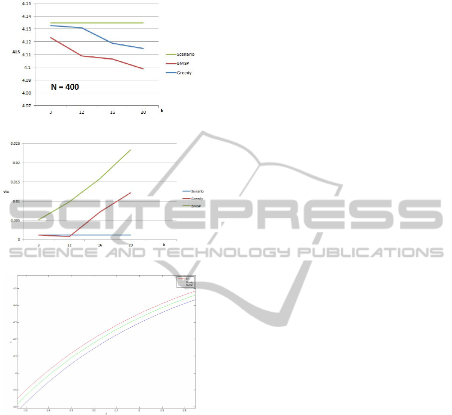
Figure 1: Comparison of average linear size for Data 1.
Figure 2: Comparison of violation ratio for Data 1.
Figure 3: Local view of chance-constrained invariant ellip-
soid of Data 1 with N = 400,k = 20.
ent values of k for 400 samples. In Figure [2], we
compare the violation of Greedy and BMSP. We ob-
serve that the increasing rate of violation is nearly the
same. Figure [3] shows the local view of ellipsoid
for Data 1 obtained by scenario approach, greedy ap-
proach and our method with N = 400 and k = 20. We
can see that the ellipsoid obtained by our method has
the smallest volume.
In Table [2], we obtain a Gap more obvious than
the previous one on Data 1. For the case where k
is chosen by (4.3.2), our method obtains a gap bet-
ter than Greedy method with 0.2% to 0.6% improve-
ment. While for other choices of k, their gap are very
close to each other.
The advantage of our method compared with
Greedy procedure is on the computing time. In the
Greedy procedure, we need to solve k + 1 times the
semidefinite program CCSP(λ) in order to decide re-
moval constrains, while in our method, we only need
to solve 2 semidefinite programs. Therefore, we ob-
serve from Table [3] that BMSP consumes much less
CPU time than Greedy and almost twice CPU time
than scenario approach. But as a counterpart of the
CPU time, we obtain better solution than scenario ap-
proach.
5 CONCLUSION
In this paper, we introduce a new simulation-based
method to solve stochastic chance constrained pro-
gram. This method is a combination of Big-M re-
laxation and a sampling-and-discarding method. We
apply this method to semidefinite programming prob-
lem in control theory. The numerical results show that
our method provides better solutions within a reason-
able CPU time.
REFERENCES
Ariyawansa, K. and Zhu, Y. (2000). Chance-constrained
semidefinite programming. Technical report, DTIC
Document.
Calafiore, G. and Campi, M. C. (2005). Uncertain convex
programs: randomized solutions and confidence lev-
els. Mathematical Programming, 102(1):25–46.
Calafiore, G. C. and Campi, M. C. (2006). The scenario
approach to robust control design. Automatic Control,
IEEE Transactions on, 51(5):742–753.
Campi, M. C. and Garatti, S. (2011). A sampling-and-
discarding approach to chance-constrained optimiza-
tion: feasibility and optimality. Journal of Optimiza-
tion Theory and Applications, 148(2):257–280.
Charnes, A., Cooper, W. W., and Symonds, G. H. (1958).
Cost horizons and certainty equivalents: an approach
to stochastic programming of heating oil. Manage-
ment Science, 4(3):235–263.
Cheung, S.-S., Man-Cho So, A., and Wang, K. (2012). Lin-
ear matrix inequalities with stochastically dependent
perturbations and applications to chance-constrained
semidefinite optimization. SIAM Journal on Opti-
mization, 22(4):1394–1430.
Dentcheva, D., Pr
´
ekopa, A., and Ruszczynski, A. (2000).
Concavity and efficient points of discrete distributions
in probabilistic programming. Mathematical Pro-
gramming, 89(1):55–77.
Garatti, S. and Campi, M. C. (2013). Modulating robustness
in control design: Principles and algorithms. Control
Systems, IEEE, 33(2):36–51.
ICORES2015-InternationalConferenceonOperationsResearchandEnterpriseSystems
80

Henrion, R. and Strugarek, C. (2008). Convexity of chance
constraints with independent random variables. Com-
putational Optimization and Applications, 41(2):263–
276.
Luedtke, J. and Ahmed, S. (2008). A sample approxima-
tion approach for optimization with probabilistic con-
straints. SIAM Journal on Optimization, 19(2):674–
699.
Nemirovski, A. (2001). Lectures on modern convex opti-
mization. In Society for Industrial and Applied Math-
ematics (SIAM. Citeseer.
Nemirovski, A. (2012). On safe tractable approximations of
chance constraints. European Journal of Operational
Research, 219(3):707–718.
Nemirovski, A. and Shapiro, A. (2006a). Convex approxi-
mations of chance constrained programs. SIAM Jour-
nal on Optimization, 17(4):969–996.
Nemirovski, A. and Shapiro, A. (2006b). Scenario ap-
proximations of chance constraints. In Probabilis-
tic and randomized methods for design under uncer-
tainty, pages 3–47. Springer.
Pagnoncelli, B. K., Reich, D., and Campi, M. C. (2012).
Risk-return trade-off with the scenario approach in
practice: a case study in portfolio selection. Journal of
Optimization Theory and Applications, 155(2):707–
722.
Pr
´
ekopa, A. (1970). On probabilistic constrained program-
ming. In Proceedings of the Princeton symposium on
mathematical programming, pages 113–138. Prince-
ton, New Jersey: Princeton University Press.
Pr
´
ekopa, A. (2003). Probabilistic programming. Hand-
books in operations research and management sci-
ence, 10:267–351.
Yao, D. D., Zhang, S., and Zhou, X. Y. (1999). LQ Control
without Riccati Equations: Stochastic Systems. FEW-
Econometrie en besliskunde.
Zhu, Y. (2006). Semidefinite programming under uncer-
tainty. PhD thesis, Washington State University.
ASamplingMethodtoChance-constrainedSemidefiniteOptimization
81
