
Model-based Clustering of Ischemic Stroke Patients
Ahmedul Kabir
1
, Carolina Ruiz
1
, Sergio A. Alvarez
2
, Nazish Riaz
3
and Majaz Moonis
3
1
Dept. of Computer Science, Worcester Polytechnic Institute, 100 Institute Road, Worcester, MA 01609, U.S.A.
2
Dept. of Computer Science, Boston College, Chestnut Hill, MA 02467, U.S.A.
3
Dept. of Neurology, Univ. Massachusetts Medical School, Worcester, MA 01655, U.S.A.
Keywords: Ischemic Stroke, EM Clustering, Gaussian Mixture Model.
Abstract: The objective of our study is to find meaningful groups in the data of ischemic stroke patients using
unsupervised clustering. The data are modeled using Gaussian mixture models with a variety of covariance
structures. Cluster parameters in each of these models are estimated by maximum likelihood via the
Expectation-Maximization algorithm. The best models are then selected by relying on information-theoretic
criteria. It is observed that the stroke patients can be grouped into a small number of medically relevant
clusters that are defined primarily by the presence of diabetes and atrial fibrillation. Characteristics of the
clusters found are discussed, using statistical comparisons and data visualization.
1 INTRODUCTION
Stroke is the rapid loss of brain function due to
disturbance in the blood supply to the brain. It is one
of the leading causes of death worldwide (Donnan et
al., 2008). Stroke can be broadly classified into two
types: Ischemic, which occurs due to lack of blood
flow; and hemorrhagic, which is caused by internal
bleeding. In this study we deal with data from
patients with ischemic stroke, the more prevalent of
the two types. The data comprises of demographic
information, medical history, laboratory test results
and treatment records of 501 patients collected
retrospectively from the University of Massachusetts
Medical School, Worcester.
Clustering is the unsupervised classification of a
set of objects into groups in such a way that objects
within a group are similar to each other based on
some perceived measure of similarity (Jain, 2010).
Clustering has been applied in many contexts and in
varied disciplines. In the field of data mining, it is
one of the major techniques for exploratory data
analysis. There are different types of clustering
algorithms. Based on the relationship between
clusters, clustering algorithms may be partitional or
hierarchical; and based on the nature of clusters they
can be centroid-based, model-based or density-based
(Pang-Ning et al., 2005).
1.1 Scope of this Paper
In this study, we attempt to find natural clusters
among stroke patients using a model-based
partitional clustering approach. Model-based
clustering is used here for its ability to produce
stable clusters along with complex models for the
clusters that can also capture correlation and
dependence of attributes (Jain and Maheswari,
2012). Finding clusters among stroke patients can be
helpful from the medical perspective as it may lead
to the discovery of new patterns and more effective
ways to manage stroke. The technique used in our
study produces two suitable clustering models – one
with two clusters and the other with three – that can
be described primarily using only two attributes:
antidiabetic medication and atrial fibrillation. Study
of the cluster assignments also revealed that there is
a clear hierarchical relation between the clusters of
the two models. The characteristics of the clusters
are analyzed by observing the attributes that have
significant differences in values between different
clusters.
1.2 Related Work
There have been numerous works that use the
technique of clustering in medical related data. One
of the studies (Bruehl et al., 1999) used cluster
analysis to validate the established diagnostic
172
Kabir A., Ruiz C., Alvarez S., Riaz N. and Moonis M..
Model-based Clustering of Ischemic Stroke Patients.
DOI: 10.5220/0005278101720181
In Proceedings of the International Conference on Health Informatics (HEALTHINF-2015), pages 172-181
ISBN: 978-989-758-068-0
Copyright
c
2015 SCITEPRESS (Science and Technology Publications, Lda.)

criteria for migraine and tension-type headache,
finding two clusters that are consistent with existing
classification. K-means clustering was used to
provide a novel approach for identifying asthma
phenotypes (Haldar et al., 2008). Later, hierarchical
clustering was used for the same purpose (Moore et
al., 2010) on a different set of patients achieving a
set of clusters with different characteristics. A
comparison of the performances of four different
clustering algorithms on clinical datasets has also
been published (Hirano et al., 2004).
Clustering has been used specifically in the field
of stroke research as well. While analyzing the effect
of stroke type on patients’ quality of life (QL),
cluster analysis was performed to identify
homogeneous subgroups of patients with specific
QL patterns (De Haan et al., 1995). The gait patterns
of patients recovering from stroke were classified
using clustering (Mulroy et al., 2003). Density-based
clustering was applied to Computed Tomography
perfusion maps to diagnose acute stroke
(Baumgartner et al., 2005). More recently, cluster
analysis has been used in stroke brainwave
classification (Omar et al., 2013) and to stratify
patients based on their motor abilities during post-
stroke recovery (Aluru et al., 2014). The
aforementioned studies apply clustering on some
specific aspects related to stroke, or in solving some
subproblems as part of a wider research. However,
to the best of our knowledge, no attempt has been
made to group stroke patients as a whole based on a
wide range of data that span from the patients’ past
medical records to medication and recovery after
stroke.
1.3 Plan of the Paper
Data preparation and clustering methodology are
described in section 2. Section 3 presents and
analyzes the results of this study. Section 4
concludes with a summary of findings and directions
for future work.
2 METHODOLOGY
2.1 Data Preparation
Our study is conducted on retrospective data
extracted from 501 records of Ischemic stroke
patients admitted at the University of Massachusetts
Medical School, Worcester, MA, USA between
2011 and 2013. Relevant information from the
medical records was extracted and collected into a
dataset after appropriate preprocessing.
2.1.1 Selection of Attributes
The attributes selected for analysis were determined
by one of the co-authors, a neurologist who
specializes in stroke medicine. The attributes include
demographic information (such as age and gender),
medical history and risk factors (such as personal
and family history of diabetes, and hypertension),
laboratory test results, and prescribed medication. A
measure of stroke severity determined by the
National Institutes of Health Stroke Scale (NIHSS)
score (Brott et al., 1989) and a measure of stroke
recovery determined by a binary categorization (see
Table 2) of the modified Rankin Scale at 90 days
after stroke (mRS-90) score (Rankin, 1957) are also
included. Among the attributes, 9 are continuous and
32 are categorical. Of the categorical attributes, only
two are multi-class and the rest are binary. A
complete list of attributes used in the study along
with summary statistics is shown in Table 1
(continuous attributes) and Table 2 (categorical
attributes).
Table 1: Summary statistics of the continuous attributes of
the stroke dataset.
Range of values Mean Standard deviation
Age 23 - 104 69.47 14.91
HbA1c 4.6 - 15 6.28 1.32
Cholesterol 85 - 400 172.76 46.26
HDL 21 - 107 46.99 14.04
LDL 11 - 415 100.93 42.30
Triglycerides 21 - 1020 130.92 93.56
BP Systolic 82 - 238 131.18 18.43
BP Diastolic 36 - 117 71.89 12.30
NIHSS score 0 - 37 6.62 7.86
2.1.2 Data Cleaning
The extraction of data from the medical records
involved a mixture of manual and automated
processing. Values of some attributes, such as lab
test results, were readily available and required no
further translation. For some other attributes, the
medical doctors co-authors of this study interpreted
the patients’ records to transform them to a suitable
value in the dataset. For example, the Infarct size of
the patient was categorized into small, medium and
large by inspecting the patients’ MRI reports.
Various commercial names of medications were
converted to their generic names. In some cases,
several attributes were aggregated into one attribute.
As an example, father, mother and sibling’s stroke
histories were combined into family history of
stroke. Spelling and abbreviation variations were
Model-basedClusteringofIschemicStrokePatients
173

also eliminated. For example, tPA, TPA, tpa and
Tissue plasminogen activator were all converted to
‘tPA’. Records with high occurrences of missing
values were omitted. Among the 501 records
included in this study, some numeric values that
remained missing (<1% overall) were replaced by
the median.
Table 2: Summary statistics of the categorical attributes of
the stroke dataset. For binary attributes, only the
percentages of TRUE values are shown. “Fam Hx” is
short for Family history; “Pre med” means medication
being used prior to stroke; and “Discharge med” are
medications present at the time of discharge from hospital.
Attribute Distribution of values
Race
White: 88.4%,
Others: 11.6%
Gender
Male: 53.3%,
Female: 46.7%
Lipid Profile Abnormal: 65.1%
Infarct Size
Small: 39.5%,
Medium: 14.6%
Large: 8.2%,
None: 37.3%
INR Abnormal: 55.9%
Hypertension 81.0%
Diabetes 30.1%
Overweight 21.4%
Smoking 19.4%
Alcohol 18.0%
Fam Hx of Stroke 13.2%
Fam Hx of Heart Disease 20.6%
Fam Hx of Cholesterol 2.6%
Fam Hx of Diabetes 8.8%
Fam Hx of Hypertension 7.4%
Previous stroke 22.4%
Coma on admission 19.0%
Atrial Fibrilation 27.7%
Active Cancer 8.6%
tPA 17.8%
Etiology of stroke
Small vessel: 15.4%,
Large vessel: 14.8%,
Cardioembolic: 31.3%
Cryptogenic: 24.2%,
Others: 6.8%
Pre med Antiplatelets 49.5%
Pre med Anticoagulants 9.2%
Pre med Statins 43.7%
Pre med Antidiabetics 22.0%
Pre med Antihypertension 66.7%
Discharge med Antiplatelets 84.8%
Discharge med Anticoagulants 18.2%
Discharge med Statins 83.2%
Discharge med Antidiabetics 23.0%
Discharge med Antihypertension 65.3%
mRS-90
Low (<3): 62.3%,
High (≥3): 37.7%
2.1.3 Attribute Preprocessing for Clustering
Since the stroke data contains attributes of different
types and ranges, steps to normalize the values were
taken. The continuous attributes were scaled to
values in the range of 0 to 1 inclusive. For each
value x in attribute A, its scaled value n
x
was
calculated by
(1)
where min
A
and max
A
are respectively the minimum
and maximum values for attribute A. For the binary
categorical attributes with true/false values, 0 and 1
were assigned to the FALSE and TRUE values
respectively. For attributes that have two possible
values Normal and Abnormal, 0 was assigned to
Normal and 1 to Abnormal. In other cases such as
gender, binary values were assigned arbitrarily to the
attribute values (0 for male, 1 for female). In the
case of multivalued categorical attributes, we took
different approaches for ordinal and non-ordinal
attributes. For the attribute infarct size, where we
have small/medium/large values with an ordinal
relationship, we assigned 0 to No infarction, 0.33 to
small, 0.66 to medium and 1 to large infarctions
respectively. For the other multivalued attribute
etiology of stroke, five binary attributes for the five
possible values were created, with each attribute
value specifying whether (1) or not (0) that
particular etiology is present in that data instance.
2.2 Clustering
Because of its simplicity, K-means (MacQueen,
1967) is often the initial technique of choice for
clustering. But K-means suffers from several
drawbacks including the requirement of pre-
selecting the number of clusters, the variability of
results for different initializations, and the
assumption of spherical equal-size clusters (Jain,
2010). As part of our study, we used K-means with
different random seeds to cluster the data with
values of k=2, 3, and 4; but the assignment of data
points to clusters varied greatly. Hence, K-means
was deemed too unstable for clustering our data.
Expectation-Maximization (EM) (Dempster et
al., 1977; Neal and Hinton, 1998) is a powerful
clustering method that uses iterative search to find
parameterized families of probabilistic models that
locally maximize the likelihood of a given set of
data. In this paper, we use the EM algorithm
initialized by hierarchical clustering for
parameterized Gaussian mixture models. We select
the clustering model by maximizing the Bayesian
Information Criterion (BIC), which provides an
optimal tradeoff between model complexity and
goodness of fit (Schwarz, 1978). To implement the
HEALTHINF2015-InternationalConferenceonHealthInformatics
174

proposed method, we wrote scripts in the R
programming language utilizing the contributed
package MCLUST (Fraley and Raftery, 2006). The
algorithm assumes a Gaussian mixture model where
the likelihood of data consisting of n observations is:
|μ
,∑
(2)
where x represents the data instances with i subscript
denoting an individual observation; G is the number
of components or clusters with k subscript
representing a particular component; τ
k
is the
probability that an observation belongs to the kth
component (or cluster); and
|
,
2
|
|
1
2
(3)
Here p is the spatial dimension (i.e., number of
attributes used for clustering); the components are
ellipsoidal, centered at the means µ
k
with covariance
matrices Σ
k
determining their other geometric
features; and each covariance matrix Σ
k
is
parameterized by eigenvalue decomposition of the
form
Σ
λ
(4)
where D
k
is the orthogonal matrix of eigenvectors,
A
k
is a diagonal matrix with its elements
proportional to the eigenvalues of Σ
k
, and λ
k
is a
scalar (Banfield and Raftery, 1993). D
k
determines
the orientation of the principal components of Σ
k
,
while A
k
determines the shape of the density
contours. λ
k
controls the volume of the
corresponding ellipsoid.
Table 3: Parameterizations of the covariance matrix Σ
k.
The three letters of the identifiers denote the volume,
shape and orientation of the distribution respectively. E, V
and I stand for Equal, Variable and Identity respectively.
For example, VEI denotes a model in which the volumes
of the clusters may vary (V), the shapes of all the clusters
are equal (E), and the orientation is the identity (I).
ID Model Distribution Volume Shape Orientation
EII λI Spherical equal equal NA
VII λ
k
I Spherical variable equal NA
EEI λA Diagonal equal equal coord. axes
VEI λ
k
A Diagonal variable equal coord. axes
EVI λA
k
Diagonal equal variable coord. axes
VVI λ
k
A
k
Diagonal variable variable coord. axes
EEE λDAD
T
Ellipsoid equal equal equal
EEV λD
k
AD
k
T
Ellipsoid equal equal variable
VEV λ
k
D
k
AD
k
T
Ellipsoid variable equal variable
VVV λ
k
D
k
A
k
D
k
T
Ellipsoid variable variable variable
Orientation, volume and shape of distributions
are estimated from the data, and can be allowed to
vary between clusters, or kept the same for all
clusters. Table 3 presents the characteristics of
different mixture models achievable by the
algorithm along with their MCLUST identifier and
corresponding equation for Σ
k
(Fraley and Raftery,
2006).
In our study, k clusters are created at each stage
starting with k = 2 and incrementing the value of k to
9. For each value of k, we try to fit ten different
clustering models as specified in Table 3. The BIC
values of all the models (including all values of k)
are compared, and the ones with highest BIC values
are chosen as our desired clustering models.
2.3 Statistical Significance of the
Differences among Clusters
Statistical hypothesis tests are used to identify
significant differences among clusters of the
distributions of individual attributes. For categorical
attributes, statistical significance is assessed by
using the χ
2
test for independence. For continuous
attributes, cluster means or medians are compared.
In the case of normally distributed attributes, a
standard ANOVA test is used for assessing
significance of differences in means. Otherwise, a
Kruskal-Wallis test (Kruskal and Wallis, 1952) is
used to assess significance of differences in
medians. The Shapiro-Wilk method (Shapiro and
Wilk, 1965) is used to test for normality.
We use the Benjamini-Hochberg method
(Benjamini and Hochberg, 1995) to control the
increased risk of false positives that is associated
with simultaneous multiple tests of significance.
Given n individual findings with corresponding
sorted p-values p
1
< p
2
< · · · < p
n
, and given a
desired overall level of significance α, the
Benjamini-Hochberg method considers as
significant only the first k findings, where k is the
largest index i, 1 ≤ i ≤ n, for which p
i
n/i < α. In this
study, the standard value of α=0.05 is our desired
level of significance. The Benjamini-Hochberg
method controls the false discovery rate (FDR), the
portion of findings that are predicted to be positives
but are actually negatives. The procedure described
here guarantees an overall FDR below the desired
level α (Benjamini and Hochberg, 1995).
Model-basedClusteringofIschemicStrokePatients
175

3 RESULTS
3.1 Selection of Clustering Models
Based on the methodology described in Section 2, a
variety of Gaussian mixture models are applied to
the dataset for different numbers (k) of clusters
where values of k are between 2 and 9. The
Bayesian Information Criterion (BIC) for each
model that could be fitted to the data is recorded, the
results of which are shown in Figure 1. The best BIC
value is achieved with the VEV model (BIC =
-15047.50) followed closely by the EEV model (BIC
= -15143.54), both of which are ellipsoid
distributions with equal shape, but differing only in
that while the former has variable volume, the latter
has same volumes. Both these models divide the
dataset into two clusters. A three-cluster VEV model
also achieves fairly good BIC value (BIC =
-15563.68). Both the spherical models EII and VII
show steady rises in BIC values as the number of
components is increased before becoming almost
constant after around k=6. We inspect the clusters
for the two-cluster VEV and EEV models and
observe that the cluster assignments are almost
identical with the exception of only two data points.
Hence for further analysis we select the VEV
models with 2 and 3 clusters respectively.
3.2 Salient Properties of the
Two-cluster Model
The two-cluster VEV mixture model creates clusters
of sizes 395 and 106 respectively. Table 4 shows the
mean and standard deviations of the continuous
attributes for each of the clusters along with their
level of significance (p-value) as determined from a
Kruskal-Wallis test which was used since all the
continuous attributes were deemed to be non-
normally distributed based on the Shapiro-Wilk test.
Table 5 shows the probability distribution of each
categorical attribute for different clusters along with
p-values computed from the χ
2
test.
Among the continuous attributes of Table 4,
HbA1c, cholesterol, HDL, LDL and Triglycerides
all have significant differences between clusters.
The first is a measure of average blood glucose level
for a prolonged period of time, while the other four
are measures of different types of fat found in the
body. What is noticeable is that the patients in
Cluster 2 exhibit lower levels of healthiness than
those of Cluster 1. On an average, Cluster 2 patients
have higher HbA1c, lower HDL (the “good”
cholesterol), higher LDL (the “bad” cholesterol) and
higher Triglyceride levels than Cluster 1 patients,
which correspond to the worse conditions for each
of these laboratory test results.
Figure 1: Comparison of BIC values for different numbers
and variations of Gaussian mixture components. Missing
points in this plot correspond to experiments that yielded
no clustering models.
Table 4: Differences in means of each continuous attribute
between clusters. The p-values that are significant after the
Benjamini-Hochberg correction at the level FDR < 0.05
are marked with an asterisk.
Attribute
Cluster 1
(395 instances)
Cluster 2
(106
instances)
Kruskal-
Wallis test
statistic
p-value
Age 69.47 ± 15.53 69.47 ± 12.29 0.065 0.7995
HbA1c 5.86 ± 0.63 7.86 ± 1.90 169.526 0.0000 *
Cholesterol 175.42 ± 44.31
162.87 ±
51.71
11.375 0.0007 *
HDL 48.14 ± 14.42 42.68 ± 11.55 13.587 0.0002 *
LDL 103.73 ± 41.82 90.48 ± 42.42 13.415 0.0002 *
Triglycerides 123.88 ± 90.33
157.15 ±
100.47
17.115 0.0000 *
BP Systolic 130.64 ± 18.06
133.16 ±
19.62
1.373 0.2413
BP Diastolic 72.30 ± 12.21 70.36 ± 12.53 1.373 0.2412
NIHSS score 6.92 ± 8.28 5.51 ± 5.93 0.016 0.9010
From Table 5, the attributes with significant
differences are in race, patients’ history of
hypertension and diabetes, and several of the
medications administered on the patient before
admission or during the time of discharge. Cluster 2
patients are more likely to be non-White, more
likely to be hypertensive and diabetic, and more
likely to be administered all of the medications than
Cluster 1 patients. The conspicuous differences
occur in the case of diabetic history and the intake of
antidiabetic medication where the probabilities for
Cluster 2 are significantly higher than Cluster 1 with
very large values of the χ
2
statistic.
Worthy of mention are some attributes that are
empirically known to be important factors for stroke
(Dyken, 1991), but exhibit no significant difference
between clusters, such as age, gender, blood
pressure, and previous history of stroke. There is
HEALTHINF2015-InternationalConferenceonHealthInformatics
176

also no significant difference in terms of stroke
severity (NIHSS score) and stroke recovery rate
(mRS-90 score).
Table 5: Differences in probabilities of each categorical
attribute between clusters. For Boolean attributes, the
probability of the TRUE value is given. The p-values that
are significant after the Benjamini-Hochberg correction at
the level FDR < 0.05 are marked with an asterisk.
Attribute
Cluster 1
(395 instances)
Cluster 2
(106 instances)
χ
2
p-value
Race (Non-White) 0.084 0.217 13.674 0.0002*
Gender (Female) 0.466 0.443 0.130 0.7188
Lipid Profile
(Abnormal)
0.648 0.660 0.452 0.7979
Infarct Size
(small/medium/
large)
0.397/ 0.137/
0.068
0.406/ 0.179/
0.132
8.131 0.0434
INR (Abnormal) 0.547 0.613 1.1028 0.5762
Hypertension 0.772 0.953 16.598 0.0000*
Diabetes 0.119 0.981 290.943 0.0000*
Overweight 0.192 0.292 4.4027 0.0359
Smoking 0.210 0.132 2.780 0.0954
Alcohol 0.195 0.123 2.494 0.1143
Fam Hx of Stroke 0.119 0.179 2.152 0.1424
Fam Hx of Heart
Disease
0.187 0.274 3.296 0.0694
Fam Hx of
Cholesterol
0.030 0.009 0.740 0.3896
Fam Hx of
Diabetes
0.076 0.132 2.623 0.1053
Fam Hx of
Hypertension
0.076 0.066 0.019 0.8908
Previous stroke 0215 0.255 0.542 0.4617
Coma on
admission
0.203 0.142 1.647 0.1993
Atrial Fibrillation 0.286 0.245 0.505 0.4772
Active Cancer 0.096 0.047 1.974 0.1600
tPA 0.195 0.113 3.282 0.0700
Etiology of stroke
(Sm ves/ Lg ves/
Card. /Crypt. /
Others)
0.144/
0.139/
0.327/
0.241/
0.063
0.189/
0.179/
0.264/
0.245/
0.085
6.1737 0.2897
Pre med
Antiplatelets
0.448 0.670 15.559 0.0000*
Pre med
Anticoagulants
0.101 0.057 1.499 0.2208
Pre med Statins 0.380 0.651 23.891 0.0000*
Pre med
Antidiabetics
0.048 0.858 315.589 0.0000*
Pre med
Antihypertensives
0.613 0.868 23.370 0.0000*
Discharge med
Antiplatelets
0.841 0.877 0.619 0.4315
Discharge med
Anticoagulants
0.182 0.179 0.000 1.0000
Discharge med
Statins
0.803 0.943 10.895 0.0010*
Discharge med
Antidiabetics
0.025 0.991 434.845 0.0000*
Discharge med
Antihypertensives
0.592 0.877 28.692 0.0000*
mRS-90
(High, ≥ 3)
0.352 0.472 4.608 0.0318
However, it is noteworthy that Cluster 1 patients
have slightly more severe stroke on average but are
more likely to have a better recovery rate. This goes
to show that the proposed clustering technique
uncovers a group of patients who are characterized
primarily by diabetes and secondarily by higher
levels of cholesterol and hypertension who are at
higher risk of poor recovery from stroke.
3.3 The Three-cluster Model and
Hierarchical Structure of Clusters
The three-cluster VEV model creates clusters
consisting of 233, 161 and 107 instances
respectively. There is a clear hierarchical structure
of clusters since the first cluster of the two-cluster
VEV model splits almost perfectly into the first two
clusters of the three-cluster model; whereas the other
cluster remains intact with the exception of only
three data points, two of which are added to and one
removed from this cluster in the three-cluster model
compared to the two-cluster model. For convenience
of understanding, we call the first two clusters 1a
and 1b and the other intact cluster 2c. We compare
the differences first between the clusters 1a and 1b
and then between all the three clusters for different
continuous (Table 6) and categorical (Table 7)
attributes. Once again the statistically significant
differences after applying Benjamini-Hochberg
correction are marked with asterisks.
In terms of the continuous attributes, the newly
formed clusters exhibit some differences in HbA1c
and some cholesterol values. The major differences,
however, are exhibited in age and stroke severity.
Patients of Cluster 1b are on an average significantly
older and suffer from more severe strokes than the
patients in Cluster 1a.
As far as the categorical attributes (Table 7) are
concerned, significant difference between the
clusters can be found in quite a few attributes.
Hypertension plays an important role in separating
these clusters as patients’ own and family history of
hypertension along with use of antihypertensive
medication are all significantly different.
Interestingly, Cluster 1a patients are more likely to
have a family history of hypertension, but are less
likely to be hypertensive themselves. Cluster 1a is
also characterized by worse health habits (more
smoking and alcohol consumption) but better
comorbid conditions (less chance of coma or atrial
fibrillation at the time of stroke). The difference
between the likelihood of atrial fibrillation in
particular is highly significant. There are also
significant differences in the use of medication,
while Cluster 1b patients have higher probability of
getting anticoagulants (blood-clot removing agents),
Cluster 1a patients are more likely to be treated with
Statins and antiplatelets during their stay at the
Model-basedClusteringofIschemicStrokePatients
177

Table 6: Differences in means for continuous attributes among clusters 1a, 1b and 2c.
Attribute
Cluster 1a
(233 instances)
Cluster 1b
(161 instances)
Cluster 2c
(107 instances)
Clusters 1a and 1b All 3 clusters
Kruskal-Wallis
statistic
p-value
Kruskal-Wallis
statistic
p-value
Age 64.27 ± 15.17 76.99 ± 12.77 69.49 ± 12.23 64.255 0.0000 * 69.939 0.0000 *
HbA1c 5.78 ± 0.60 5.96 ± 0.66 7.86 ± 1.88 7.086 0.0078 * 181.748 0.0000 *
Cholesterol 182.64 ± 43.79 164.45 ± 42.90 163.78 ± 51.76 18.630 0.0000 * 27.627 0.0000 *
HDL 48.43 ± 14.36 47.71 ± 14.53 42.75 ± 11.53 0.540 0.4623 13.647 0.0011 *
LDL 107.48 ±38.96 97.77 ± 44.96 91.41 ± 42.77 9.571 0.0020 * 20.942 0.0000 *
Triglycerides 137.69 ± 104.10 104.06 ± 60.50 156.60 ± 100.16 15.340 0.0000 * 32.474 0.0000 *
BP Systolic 129.00 ± 16.46 133.07 ± 19.99 133.06 ± 19.51 2.948 0.0860 4.198 0.1226
BP Diastolic 73.10 ± 11.60 70.86 ± 12.98 70.79 ± 12.48 2.994 0.0836 3.600 0.1653
NIHSS score 4.39 ± 5.72 10.45 ± 9.76 5.73 ± 6.41 38.503 0.0000 * 40.5951 0.0000 *
Table 7: Differences in probabilities for continuous attributes among clusters 1a, 1b and 2c.
Attribute
Cluster 1a
(233 instances)
Cluster 1b
(161 instances)
Cluster 2c
(107 instances)
Clusters 1a and 1b All 3 clusters
χ2 p-value χ2 p-value
Race (Non-White) 0.099 0.062 0.215 1.219 0.2695 15.873 0.0004 *
Gender (Female) 0.451 0.484 0.449 0.569 0.4505 0.860 0.6505
Lipid Profile (Abnormal) 0.661 0.627 0.664 2.234 0.3272 2.719 0.6058
Infarct Size
(small/medium/large)
0.412 / 0.150 /
0.52
0.373/0.118
/ 0.093
0.411 / 0.178
/0.131
3.718 0.2936 11.429 0.076
INR (Abnormal) 0.524 0.578 0.607 1.156 0.561 2.471 0.6499
Hypertension 0.717 0.851 0.953 8.9815 0.0027 * 29.236 0.0000 *
Diabetes 0.086 0.161 0.981 4.576 0.0324 301.305 0.0000 *
Overweight 0.227 0.143 0.290 3.852 0.0497 8.755 0.0126 *
Smoking 0.270 0.118 0.140 12.505 0.0004 * 16.646 0.0002 *
Alcohol 0.245 0.124 0.121 8.030 0.0046 * 12.4887 0.0019 *
Fam Hx of Stroke 0.142 0.087 0.178 2.214 0.1368 4.987 0.0826
Fam Hx of Heart Disease 0.249 0.093 0.280 14.288 0.0002 * 18.802 0.0000 *
Fam Hx of Cholesterol 0.047 0.006 0.009 4.120 0.0424 7.8159 0.0201 *
Fam Hx of Diabetes 0.099 0.043 0.131 3.381 0.0659 6.789 0.0339 *
Fam Hx of Hypertension 0.124 0.006 0.065 17.283 0.0000 * 19.607 0.0000 *
Previous stroke 0.215 0.211 0.262 0.000 1.0000 1.146 0.5638
Coma on admission 0.137 0.292 0.150 13.245 0.0003 * 16.230 0.0003 *
Atrial Fibrilation 0.013 0.683 0.243 205.907 0.0000 * 214.231 0.0000 *
Active Cancer 0.107 0.081 0.047 0.496 0.4814 3.506 0.1732
tPA 0.137 0.267 0.131 9.574 0.0020 * 13.011 0.0015 *
Etiology of stroke (Sm
ves/ Lg ves/ Card. /Crypt.
/ Others)
0.227/0.210/
0.043/ 0.399/
0.107
0.025/0.037/
0.733/0.006/
0.000
0.187/0.178/
0.271/ 0.252/
0.084
302.895 0.000* 317.047 0.0000 *
Pre med Antiplatelets 0.408 0.509 0.664 3.572 0.0588 19.392 0.0000 *
Pre med Anticoagulants 0.030 0.199 0.065 28.525 0.0000 * 33.638 0.0000 *
Pre med Statins 0.365 0.410 0.636 0.6406 0.4235 22.552 0.0000 *
Pre med Antidiabetics 0.017 0.099 0.841 11.703 0.0006 * 310.515 0.0000 *
Pre med
Antihypertensives
0.528 0.745 0.850 18.137 0.0000 * 40.942 0.0000 *
Discharge med
Antiplatelets
0.944 0.689 0.879 44.126 0.0000 * 48.986 0.0000 *
Discharge med
Anticoagulants
0.039 0.391 0.178 76.951 0.0000 * 79.685 0.0000 *
Discharge med Statins 0.893 0.671 0.944 28.145 0.0000 * 45.733 0.0000 *
Discharge med
Antidiabetics
0.034 0.000 1.000 4.0484 0.0442 457.318 0.0000 *
Discharge med
Antihypertensives
0.567 0.634 0.869 1.506 0.2197 30.010 0.0000 *
mRS-90 (High, ≥ 3) 0.219 0.547 0.467 43.355 0.0000 * 48.216 0.0000 *
hospital. Etiology (cause) of stroke also shows an
interesting pattern: Cardioembolic strokes are
prevalent in Cluster 1b while all other etiologies are
more associated with Cluster 1a. A striking
HEALTHINF2015-InternationalConferenceonHealthInformatics
178
difference between the two clusters is in stroke
recovery rate where Cluster 1a patients are much
more likely to recover well from stroke.
If we compare all the three clusters together,
many attributes show significant differences
between clusters. The ones that stand out are
diabetes along with pre and discharge med
antidiabetics, atrial fibrillation, and etiology of
stroke. Age, NIHSS score, mRS-90 score, and
discharge medications of antiplatelets,
anticoagulants and Statins also display highly
significant differences.
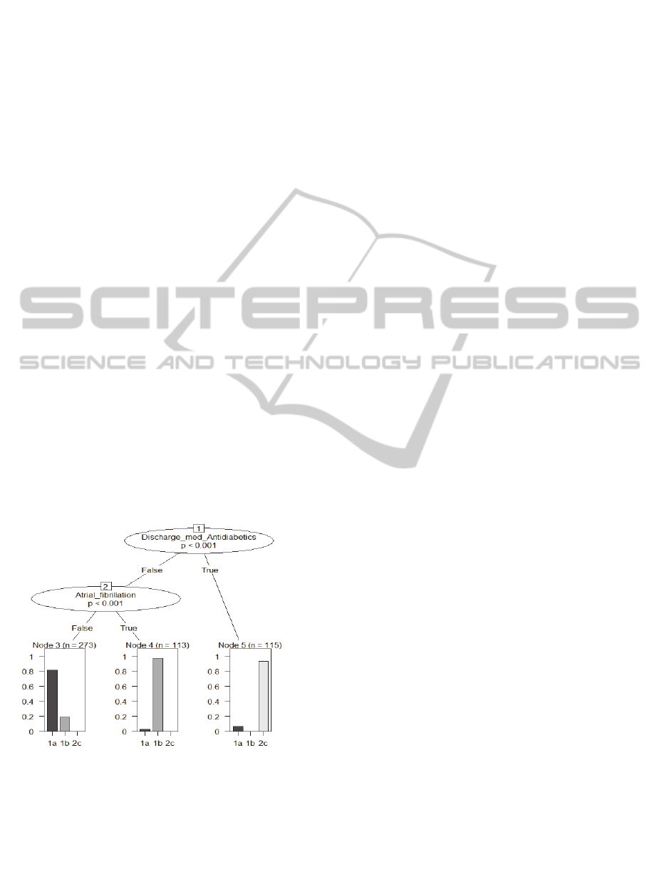
3.4 Decision Tree to Predict Clusters
From the three-cluster model, we build a decision
tree where all the attributes of the dataset are used as
the predicting variables and the assigned cluster for
each record is used as the target (prediction)
attribute. The C4.5 algorithm (Quinlan, 1996) is
used, as implemented in the J4.8 function in Weka
(Witten et al., 2011), with a pruning confidence
factor of 0.01 and a minimum of 40 instances per
leaf to achieve a minimalist tree with only two inner
nodes and three leaves. The resulting tree, shown in
Figure 2, has accuracy = 87.62%, precision = 0.890,
recall = 0.876 and area under the ROC curve = 0.887
evaluated by 10-fold cross-validation. Using only
two attributes - discharge medication of antidiabetics
and comorbid condition of atrial fibrillation - the
three clusters can be defined reasonably accurately.
Figure 2: Decision tree to predict cluster assignments.
3.5 Cluster Visualization
We now present a series of plots visualizing the data
clusters created by our proposed methods. In each
plot a pair of attributes with significant differences
across clusters are chosen, and their cluster
assignments are shown. Figure 3 shows the cluster
assignments with respect to the risk factors diabetes
and hypertension for both the two-cluster and three-
cluster models. The ellipses show the cluster centers
with the axes representing the within cluster
covariance. A small amount of random noise (jitter)
was added to the attribute values to separate the data
points that would otherwise be in the same
coordinate. In Figure 3(a), there is clear separation
between clusters 1 and 2 based on diabetes. In
Figure 3(b), Cluster 2c stays in the same place as
Cluster 2, whereas Cluster 1 breaks into overlapping
clusters 1a and 1b based on hypertension.
If we take a look at a pair of continuous
attributes Age and HbA1c in Figure 4, we see a
similar structure where Clusters 1 and 2 are
separated by HbA1c and not Age (Figure 4a), but in
the split clusters 1a and 1b show significant
differences in age. The values of both the attributes
are normalized to a [0,1] range.
The hand-picked dimensions selected in Figures
3 and 4 to project the clustered data onto provide a
good visual separation of the clusters. Interestingly,
the two dimensions suggested by the decision tree in
Section 3.4, Discharge Med Antidiabetics and Atrial
fibrillation, provided a much better projection space
to discern the three clusters. The jitter-added data
points for these attributes are shown in Figure 5, and
clearly demonstrate well-defined clusters described
by these two attributes.
4 CONCLUSIONS
This paper has presented the results of clustering
stroke patients based on the data consisting of
demographics, medical history, test results and
medication records. Using the EM algorithm to
estimate the parameters of Gaussian mixture models,
two suitable clustering schemes are found that
suggest the division of the stroke patients into two
and three clusters respectively. With two attributes -
antidiabetic medication at discharge and atrial
fibrillation – selected by a decision tree constructed
over the clustered data, the clusters can be well
discerned. A hierarchical structure between the two-
cluster and three-cluster structure is observed and
the nature of the relationship among clusters
uncovered. Statistically significant differences in the
values of various attributes across clusters are found
and examined.
The clusters present very interesting patterns
from a medical perspective. In the two-cluster
model, the clusters can be described almost entirely
Model-basedClusteringofIschemicStrokePatients
179
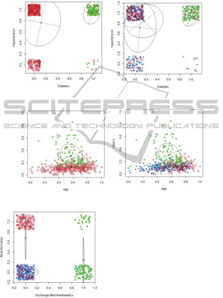
(a) (b)
Figure 3: Clustered data projected onto Diabetes and Hypertension for a) Two-cluster and b) Three-cluster models.
(a) (b)
Figure 4: Clustered data projected onto Age and HbA1c for a) Two-cluster and b) Three-cluster models.
Figure 5: Clustered data projected onto Discharge Med
Antidiabetics and Atrial Fibrillation.
by the history of diabetes and use of antidiabetic
medicine.
The cluster characterized by the high presence of
diabetes also exhibits poor conditions of
hypertension and body fat levels. In the three-cluster
model, this cluster stays almost unchanged while the
other cluster splits into two new clusters which are
separated primarily by atrial fibrillation. One of
these clusters represent older patients with more
severe conditions at the time of stroke, and
significantly lower rate of recovery. The other
cluster is characterized by younger patients with
poorer health habits (more smoking and alcohol
consumption), but nevertheless exhibiting less
severe strokes and more favorable outcomes after
stroke. Interestingly the mRS-90 score, a medical
outcome measuring stroke recovery after 90 days of
1
1a
1b
1
1a
1b
2
2
2c
2c
HbA1c
2c
1a
1b
HEALTHINF2015-InternationalConferenceonHealthInformatics
180

stroke onset, varies significantly among the three
clusters. This provides additional evidence that
further thorough analysis of these clusters from a
medical point of view may lead to better
understanding of stroke physiology and more
informed management of stroke patients.
Furthermore, the information from these clusters
may be utilized to address other research problems,
such as the construction of computational models for
identifying people at risk of stroke, and for
predicting the outcome of patients after stroke.
REFERENCES
Aluru, V., Lu, Y., Leung, A., Verghese, J. and Raghavan,
P., 2014. Effect of auditory constraints on motor
performance depends on stage of recovery post-stroke.
Frontiers in neurology, 5.
Banfield, J. D. and Raftery, A. E., 1993. Model-based
Gaussian and non-Gaussian clustering. Biometrics,
pp.803-821.
Baumgartner, C., Gautsch, K., Böhm, C. and Felber, S.,
2005. Functional cluster analysis of CT perfusion
maps: a new tool for diagnosis of acute stroke?.
Journal of digital imaging, 18(3), pp.219-226.
Benjamini, Y. and Hochberg, Y., 1995. Controlling the
false discovery rate: a practical and powerful approach
to multiple testing. Journal of the Royal Statistical
Society. Series B (Methodological), pp. 289-300.
Brott, T., Adams, H. P., Olinger, C. P., Marler, J. R.,
Barsan, W. G., Biller, J., Spilker, J., Holleran, R.,
Eberle, R. and Hertzberg, V., 1989. Measurements of
acute cerebral infarction: a clinical examination
scale. Stroke, 20(7), pp.864-870.
Bruehl, S., Lofland, K. R., Semenchuk, E. M., Rokicki, L.
A. and Penzien, D. B., 1999. Use of Cluster Analysis
to Validate IHS Diagnostic Criteria for Migraine and
Tension Type Headache. Headache: The Journal of
Head and Face Pain, 39(3), pp.181-189.
De Haan, R. J., Limburg, M., Van der Meulen, J. H. P.,
Jacobs, H. M. and Aaronson, N. K., 1995. Quality of
life after stroke impact of stroke type and lesion
location. Stroke, 26(3), pp.402-408.
Dempster, A. P., Laird, N. M. and Rubin, D. B., 1977.
Maximum likelihood from incomplete data via the EM
algorithm. Journal of the Royal Statistical Society.
Series B (Methodological), pp.1-38.
Donnan, G. A., Fisher, M., Macleod M., Davis, S.M.,
2008, Stroke, The Lancet 371 (9624).
Dyken, M. L., 1991. Stroke risk factors. In Prevention of
stroke, pp. 83-101. Springer New York.
Fraley, C. and Raftery, A. E., 2006. MCLUST version 3:
an R package for normal mixture modeling and
model-based clustering. Washington Univ Seattle Dept
of Statistics.
Haldar, P., Pavord, I. D., Shaw, D. E., Berry, M. A.,
Thomas, M., Brightling, C. E., Wardlaw, A. J. and
Green, R. H., 2008. Cluster analysis and clinical
asthma phenotypes. American journal of respiratory
and critical care medicine, 178(3), pp.218-224.
Hirano, S., Sun, X. and Tsumoto, S., 2004. Comparison of
clustering methods for clinical databases. Information
Sciences, 159(3), pp.155-165.
Jain, A. K., 2010. Data clustering: 50 years beyond K-
means. Pattern Recognition Letters,
31(8), pp.651-
666.
Jain, A. K. and Maheswari, S., 2012. Survey of recent
clustering techniques in data mining. Int. J. Comput.
Sci. Manage. Res, 1, pp.72-78.
Kruskal, W. H. and Wallis, W. A., 1952. Use of ranks in
one-criterion variance analysis. Journal of the
American statistical Association, 47(260), pp.583-621.
MacQueen, J., 1967. Some methods for classification and
analysis of multivariate observations. In Proceedings
of the fifth Berkeley symposium on mathematical
statistics and probability (Vol. 1, No. 14, pp. 281-
297).
Moore, W. C., Meyers, D. A., Wenzel, S. E., Teague, W.
G., Li, H., Li, X., ... and Bleecker, E. R., 2010.
Identification of asthma phenotypes using cluster
analysis in the Severe Asthma Research
Program. American journal of respiratory and critical
care medicine, 181(4), pp.315-323.
Mulroy, S., Gronley, J., Weiss, W., Newsam, C. and
Perry, J., 2003. Use of cluster analysis for gait pattern
classification of patients in the early and late recovery
phases following stroke. Gait & posture, 18(1),
pp.114-125.
Neal, R. M. and Hinton, G. E., 1998. A view of the EM
algorithm that justifies incremental, sparse, and other
variants. Learning in graphical models. Springer
Netherlands, pp.355-368.
Omar, W. R. W., Taib, M. N., Jailani, R., Fuad, N., Isa, R.
M., Jahidin, A. H. and Sharif, Z., 2013. Acute
Ischemic Stroke Brainwave Classification Using
Relative Power Ratio Cluster Analysis. Procedia-
Social and Behavioral Sciences, 97, pp.546-552.
Pang-Ning, T., Steinbach, M. and Kumar, V., 2005.
Introduction to data mining. Addison-Wesley. 2
nd
edition.
Quinlan, J. R., 1996, Improved use of continuous
attributes in C4.5. Journal of Artificial Intelligence
Research, 4:77-90.
Rankin, J., 1957. Cerebral vascular accidents in patients
over the age of 60. II. Prognosis. Scottish medical
journal, 2(5), pp.200-215.
Schwarz, G., 1978. Estimating the dimension of a model.
The annals of statistics, 6(2), pp.461-464.
Shapiro, S.S. and Wilk, M.B., 1965. An analysis of
variance test for normality (complete samples).
Biometrika, pp.591-611.
Witten, I. H., Frank, E. and Hall, M. A., 2011. Data
Mining: Practical Machine Learning Tools and
Techniques. Morgan Kaufmann. 3
rd
edition.
Model-basedClusteringofIschemicStrokePatients
181
