
Classification of Involuntary Hand Movements
Aki H
¨
arm
¨
a
Philips Research, Eindhoven, The Netherlands
Keywords:
Involuntary Movements, Autoregressive Modeling, Pattern Recognition, Hidden Markov Model.
Abstract:
Involuntary movements of arms and legs reflect neural and metabolic processes in the human body. In this
paper the focus is on the properties of physiological tremor, shivering, and tremors caused by physical fatigue
measured in fingers of a subject. Three different signal modeling paradigms are compared in the paper using
accelerometer data. It is first demonstrated that the data can be modeled as a nearly stationary low-order AR
process. Next, it is shown that the different data types can be classified using long-term feature distributions
in a naive Bayes classifier. Finally, a comparable performance is obtained when the signal is modeled as a
Markov process emitting small prototypical movements or jerks.
1 INTRODUCTION
Involuntary movements are common in all animals
and typical symptoms in fever, Parkinson’s disease,
diabetes, and many other medical conditions. The
movements may originate from many different pro-
cesses in the body. Therefore, one may assume that
the classification of the movements could be used
to get information about the medical state of a pa-
tient. Typical diagnostic tools are various types of
tests (Watts et al., 2011), electromyography (Palmes
et al., 2010), and movement sensors (Wyatt, 1968;
Ackmann et al., 1977) such as accelerometers which
are used in the current paper.
The muscular system is organized largely as pairs
of antagonist muscles. In normal operation the mus-
cular system is excited by many different processes
and even the basic control of a steady posture is
the result of active stochastic excitation of individual
muscle bundles and feedback via the sensory system.
Computational neuromusculoskeletal models (Zhang
et al., 2009; Yao et al., 2012) show that the system has
an inherent tendency to oscillate. A consequence of
this continuous activity is physiological tremor which
is present in all organisms with a muscular system. In
this paper the focus is on physiological tremor, shiv-
ering, and tremors caused by muscle fatigue.
A lowered body temperature triggers the ther-
moregulatory system to activate muscles to produce
extra heat and this leads to shivering of the body. The
actual mechanism of shivering is not well understood
but it is considered to be driven by bursts of neural
activity from the rostral ventromedial medulla in the
brain through the sympathetic nervous system (Mor-
rison and Nakamura, 2011). Sung et al (Sung et al.,
2004) demonstrated that the shivering can be detected
from an accelerometer attached to the body and the
classification of movement patterns can be used to
get a rough estimate of the core body temperature.
Physical stress in muscles causes fatigue which often
leads to tremors. These movements are often associ-
ated with metabolic processes in the motor cells in the
muscles themselves (Ebenbichler et al., 2000).
In signal analysis and classification the goal is to
identify the underlying process behind the observed
data. In many areas, e.g., speech processing, signal
models that are based on functional models of the pro-
cess have been found successful. Detailed neuromus-
culoskeletal models of hand movements have been in-
troduced, e.g., in (Akamatsu et al., 1988; Zhang et al.,
2009; Yao et al., 2012), but they do not have an in-
vertible signal model and they also contain parame-
ters that are typically not available and therefore do
not directly lead to a practical signal analysis method-
ology. The problem of the modeling of involuntary
hand movements for classification is a central topic
of this paper and an area where little systematic work
from signal modeling perspective has been done in
the past. Physiological tremors, shivering and tremors
caused by muscle fatigue seem to have different ori-
gins which makes them interesting for this study. In
fact, the current author is not aware of a previous com-
parison of those three common types of movements in
the same experimental setting.
312
Härmä A..
Classification of Involuntary Hand Movements.
DOI: 10.5220/0005280503120317
In Proceedings of the International Conference on Bio-inspired Systems and Signal Processing (BIOSIGNALS-2015), pages 312-317
ISBN: 978-989-758-069-7
Copyright
c
2015 SCITEPRESS (Science and Technology Publications, Lda.)
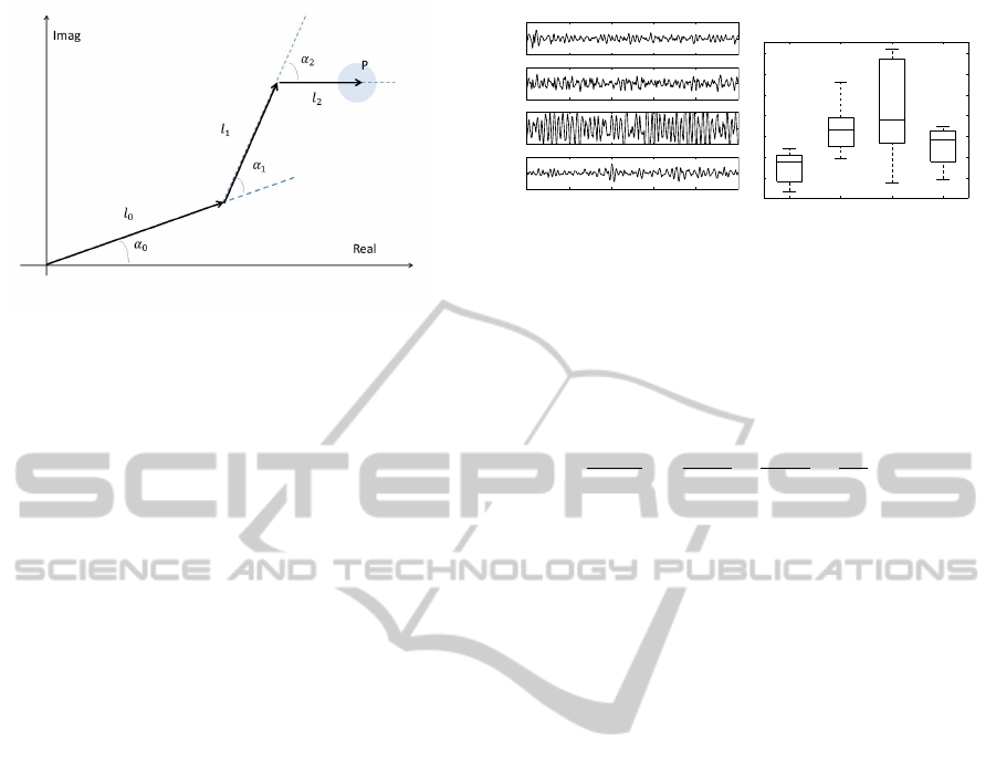
Figure 1: Simplified model of the arm, hand, and finger in
a plane.
The three basic signal modeling paradigms are
source-filter modeling, distribution models, and se-
quential models. We start with short discussion on
kinematic modeling of hand movement and introduce
the experimental data collected for this paper. Next,
for each of the three modeling paradigms we define
and motivate the methodology, and provide results of
the experiments with the data. Finally, the paper is
concluded by a discussion on the results and recom-
mendations for future work in the analysis of involun-
tary hand movements.
2 SIGNAL MODELS
A simplified geometric model of arm and hand in a
complex 2D plane is illustrated in Fig. 1. With the
origin in the root of the arm, the position of the tip of
the finger, P, can be expressed by
p(t) =
J−1
∑
j=0
l
j
e
−i
∑
j
k
(α
k
(t))
(1)
where J is the number of joints and l
j
and α
j
are the
bone lengths and joint angles, respectively. The joint
angles change due to the contractions of the muscles
connected over the joint which are caused by neural
excitation in the muscle bundles. The movement of
the hand (and the captured signal from an accelerom-
eter) is therefore driven by multiple neural source sig-
nals. The arrival times of individual impulses in dif-
ferent muscles are probably uncorrelated but the sig-
nals may still have some long-term correlations. The
model does not contain the effects of inertia, elasticity
of the muscles, and the neural feedback.
The minimum jerk model by Flash and Hogan
(Flash and Hogan, 1985) is a simplified model for the
kinematics of a short linear movement of a hand from
a rest at the position x
0
to full stop at x
f
in time t
f
.
The position as a function of time is given by
x(t) = x
0
+ (x
0
− x
f
)(15τ
4
− 6τ
5
− 10τ
3
) (2)
−0.5
0
0.5
−0.5
0
0.5
−0.5
0
0.5
0 1 2 3 4 5
−0.5
0
0.5
TIME [s]
REST COLD STRESS RECOVERY
−40
−35
−30
−25
−20
−15
−10
AMPLITUDE [dB]
Figure 2: Left: Fragments of rest, cold, stress, and recov-
ery, from top to bottom, respectively. Right: median and
quartile RMS values of signals over all data.
where τ = t/t
f
. For the purpose of this paper one
may notice that the measured acceleration h(t) cor-
responds to the second derivative of the function and
it is given by
h(t) =
d
2
x(t)
dt
2
= (
180t
2
t
4
f
−
120t
3
t
5
f
−
60t
t
3
f
)(x
0
− x
f
)
(3)
The model has no biometric parameters like bone
lengths or masses which would be difficult to acquire.
Assuming that the movements in three directions are
independent it can be directly extended to 3D ac-
celerometer data.
3 EXPERIMENTAL DATA
The goal of the experiment was to compare the three
different signal modeling paradigms with realistic
data. The data set was collected using a 3-axis ac-
celerometer (Xsens MTx) which was attached on the
back of the middle and ring finger of the subject us-
ing an elastic band. The data was captured at the sam-
pling rate of 100 Hz. The physiological tremors were
measured in an office room with the subject sitting
and resting the elbow on the corner of a desk. Next,
the subject went outdoors without a coat (temperature
was around 0
◦
C) and stood there for 2-4 minutes until
the subject was clearly shivering or wanted to stop the
experiment. Next, after a short rest and warming, the
subject held a 1-3kg weight in the hand arm extended
to the front until the subject felt the fatigue in the arm
and/or could not hold the weight anymore. After the
period of physical stress the subject was resting until
the perceived fatigue disappeared. The data was con-
sequently segmented to four parts: rest, cold, stress,
and recovery. Five healthy male subjects participated
in the data collection. Waveforms from the different
classes are illustrated in Fig. 2. A dominant frequency
component around 10Hz can be often found but there
are large individual differences.
The accelerometer signals were preprocessed by a
ClassificationofInvoluntaryHandMovements
313

steep high-pass filter with a cutoff at 2Hz to remove
the effects of slow hand movements and gravity from
the data.
4 SOURCE-FILTER MODEL
One may consider h(t) in (3) as the impulse response
of the system from a single neural impulse to the ob-
served accelerometer data. As a source-filter model it
may be written in the following form:
a(t) =
∞
∑
k=0
M
∑
m=1
h
m
(k,t)e
m
(t − k) (4)
where M is the number of muscles contributing to
the movements, h
m
(k,t) is the time-varying kinematic
impulse response from an mth muscle (or j th joint
in the geometric model) to the accelerometer signal,
and e
m
(t) is the neural source signal (Vinjamuri et al.,
2009) exciting the muscle. This is a linear approxima-
tion which assumes that the effects of the muscles are
independent. In the case of small movements the lin-
earization and independence assumption can be con-
sidered justifiable.
Low-order autoregressive models have been used
earlier in the spectrum analysis of hand tremors
(Zhang and Chu, 2005; Becker et al., 2008; Kucukel-
bir et al., 2009). Several authors, e.g., (Gantert et al.,
1992) have used measures based on the predictabil-
ity of phase space trajectories (e.g., Lyapunov expo-
nents) to model tremors. In (Vinjamuri et al., 2009)
the signals from multiple accelerometers were mod-
eled as convolutive mixtures of a neural source signals
that are exciting the muscles. They used independent
component analysis to extract the hypothetical neural
source signals. The assumed signal model each sen-
sor was therefore similar to (4).
The signal model (4) has multiple source signals
which each have a different impulse response which
makes the modeling problem very difficult. Let us as-
sume that the excitation is sparse such that at a move-
ment is predominantly caused by one neural source
signal or a muscle. In this case, the model of (4)
could be approximated by a time-varying autoregres-
sive model given by
a(t) =
∞
∑
k=0
h(k,t)e(t − k) (5)
where h(k,t) is a time-varying impulse response
switching between the different input terminals of the
neural source signal. The sparsity assumption has no
obvious biomechanical evidence but it is a plausible
assumption at least for single rapid jerks.
REST COLD STRESS RECOVERY
0
2
4
6
8
10
12
14
16
18
20
PREDICTION GAIN [dB]
Figure 3: Prediction gain values averaged over all subject
and data. The G
p
values of the stationary AR model are
shown by triangles.
In this paper the time-varying AR system is mod-
eled using the time-varying autoregressive (TVAR)
method by Grenier (Grenier, 1983). It is essentially
similar to Burg’s lattice algorithm (AR) but replaces
stationary reflection coefficients by sums of time-
varying basis functions (in this case, sigmoids). The
time-varying reflection coefficients of the estimated
Grenier’s model represent the kinematic impulse re-
sponses and the prediction residual signal e(t) models
the neural excitation. The performance of the source-
filter model can be characterized by the prediction
gain given by G
p
= 20 log
10
(E[|a(t)|
2
]/E[|e(t)|
2
]).
The prediction gain values of the 8th order Grenier’s
model estimated in 10s frames averaged over all sub-
jects are shown in Fig. 3. Shivering seems to give the
largest median G
p
value and there is clear difference
to the stress condition. Fig. 2 shows that the RMS
values of those conditions do not differ significantly.
The difference between rest and cold conditions how-
ever may be related to the difference in RMS values.
Shivering seems to be more predictable than tremors
caused by stress. The TVAR model gives consistently
a 2-4dB advantage over the static Burg AR model
(triangles) in other than the stress condition. Addi-
tional experiments demonstrated that the G
p
in both
AR and TVAR does not increase when the model or-
der is higher that 6. Therefore, one may conclude that
data can be modeled as a mildly time-varying low-
order AR process and especially the stress condition
seems to differ in predictability and time-variability
from the other conditions.
5 DISTRIBUTION MODELING
It is common to assume that underlying process is
ergodic such that the long-term statistics of features
BIOSIGNALS2015-InternationalConferenceonBio-inspiredSystemsandSignalProcessing
314

computed from the data are similar over time and in
different subjects. For example, in (Jakubowski et al.,
2002) the higher-order statistics features computed
from accelerometer data were used in a feed-forward
neural network to classify successfully physiological,
Parkinson’s, and essential tremor data.
In early experimentation with multiple algorithm
candidates the naive Bayes classifier turned out to be
one of the most efficient methods for this type of data.
A set of F time- and frequency domain features were
computed in one second frames of acceleration data.
The naive Bayes model assumes that individual fea-
tures are conditionally independent random variables
within each class, see (Murphy, 2012). The distribu-
tion p
f
(x|c) of the feature f values within each class c
is estimated from the training data. For the unknown
input feature vector x
¯
the likelihood value for each
class c are given by
p(x
¯
|c) =
F−1
∏
f =0
p
f
(x|c) (6)
and choose the class that gives the maximum value.
This is a probabilistic signal model that characterizes
the long-term statistics of the features computed from
the signal.
The following features were computed in two sec-
ond segments from the data: normalized signal vari-
ance, ratio between maximum and mean absolute val-
ues, maximum frequency, prediction gain G
p
, and the
first four cepstrum coefficients computed on a near-
logarithmic frequency scale. The naive Bayes classi-
fier was trained using the data from the four classes.
The experiment was performed using repeated leave-
one-out cross-validation so that the model was tested
always using the data from one subject who was not
included in the training data. The accumulated sensi-
tivity and specificity percentages over all four classes
were 80 and 70%, respectively. The largest number
of classification errors was between rest and recovery
periods which suggest that most subjects recovered
very quickly.
6 SEQUENTIAL MODELS
The kinematic model above suggests that the move-
ment data consists of a sequence of individual events,
jerks and spasms. The proposed signal model corre-
sponding to J such jerks is given by
a(t) =
J
∑
j
h
j
(t −t
j
) (7)
where h
j
(t) is the function of (3) defined in the inter-
val [0,t
f
( j)] and zero otherwise. The length of the in-
terval t
f
( j) (as well as x
0
and x
f
) depends on j but it is
likely that there are often similar recurring jerks in the
data so that the data can be approximated effectively
by a limited alphabet of prototypical jerks. Therefore,
one may approximate the signal model (6) by a sys-
tem that produces a sequence of timed indexes of pro-
totypical movements from a fixed vocabulary. For this
type of data it is natural to use hidden Markov mod-
els (HMM), conditional random fields (CRF), or other
graphical models. Sung et al (Sung et al., 2004) used
the HMM in the method for the analysis of shivering.
Their results were promising but they did not give a
clear motivation why shivering was considered as a
Markov process. The discrete HMM model models
state transitions in a hidden state machine where only
the emissions of this state machine at each state transi-
tion are observable. One may associate the emissions
with the individual movements in the accelerometer
data and the hidden state machine with the underly-
ing processes in the body.
A practical way to create the vocabulary of move-
ments, or jerks, is to initialize a codebook of candi-
date functions and then search for a limited vocabu-
lary of J jerk patterns that has the best match with
the data. This was performed using a matching pur-
suit search with functions of the Flash-Hogan model
(3) which are characterized by the duration t
f
and
the excursion x
f
, respectively. The matching crite-
ria is the Euclidean distance between the accelerom-
eter data segment represented by a zero-mean vector
a(t) and a movement vector h(x
f
,t
f
) of (3), where t
is the time index corresponding to the first element of
the vector and length of the vector is the same as the
length of h(x
f
,t
f
). In order to compare different can-
didate functions the value is convenient to convert in
to a score value in range [0,1]. This is given by
s(t,x
f
,t
f
) = max(0,1 − |a(t) − h(x
f
,t
f
)|
2
/|a(t)|
2
).
(8)
For example, Figure 4 shows examples of average
score values for different types of movement data in
one subject. One can pick a number of local maxima
from each figure as the most typical cases of move-
ments in the data characterized by the excursion x
f
and the duration t
f
. This was repeated for the entire
data set and then a subset of Flash-Hogan functions
was determined by searching the maxima within each
local connected region in the obtained figure. The ac-
celerometer data is converted to a sequence of pro-
totype indices so that in each short time segment the
prototype vector that gives the maximum score is se-
lected. The parameter values for eight common jerk
patters were selected from the data. In the experi-
ments the winning prototype giving the highest score
was selected in non-overlapping segments of 100ms
ClassificationofInvoluntaryHandMovements
315

REST
EXCURSION [mm]
100 200 300 400 500
1
2
3
4
5
SHIVERING
100 200 300 400 500
1
2
3
4
5
STRESS
TIME [ms]
EXCURSION [mm]
100 200 300 400 500
1
2
3
4
5
RECOVERY
TIME [ms]
100 200 300 400 500
1
2
3
4
5
Figure 4: Average score values for the data from one subject
(black color - score 1.0).
leads to a data rate of 10 prototype indices per sec-
ond. The training and cross-validation of the HMM
were performed in the same way as in Section 5. The
model had 12 hidden states and the model for tested
for each 4 second episode.
The accumulated results of multiple cross-
validations show that the sensitivity and specificity of
the HMM model in the four-class classification prob-
lem are 75% and 75%, respectively, and the largest
errors are again in the correct classification of the re-
covery phase.
7 DISCUSSION
The topic of the paper is automatic classification of
physiological tremor, shivering, and tremors caused
by physical stress. Three different experiments were
reported. First, it was demonstrated that the ac-
celerometer data can be modeled as a low-order time-
varying autoregressive process and that there are dif-
ferences between the data types in the prediction gain
values. Next, the experiment with a naive Bayes clas-
sifier showed that the different data types can be clas-
sified based on long-term statistics. Finally, similar
classification performance was obtained by modeling
movements as a Markov process of small prototypic
movements.
All modeling approaches seem motivated and are
effective but the error rates were relatively high in all
classification experiments, in particular, in the recov-
ery and resting data.
REFERENCES
Ackmann, J. J., Sances, A., Larson, S. J., and Baker, J. B.
(1977). Quantitative Evaluation of Long-Term Parkin-
son Tremor. Biomedical Engineering, IEEE Transac-
tions on, BME-24(1):49–56.
Akamatsu, N., Hannaford, B., and Stark, L. (1988). An
intrinsic mechanism for the oscillatory contraction
of muscle. In Engineering in Medicine and Biol-
ogy Society, 1988. Proceedings of the Annual Inter-
national Conference of the IEEE, pages 1730–1731
vol.4. IEEE.
Becker, B. C., Tummala, H., and Riviere, C. N. (2008). Au-
toregressive modeling of physiological tremor under
microsurgical conditions. In Engineering in Medicine
and Biology Society, 2008. EMBS 2008. 30th Annual
International Conference of the IEEE, pages 1948–
1951. IEEE.
Ebenbichler, G. R., Kollmitzer, J., Erim, Z., L
¨
oscher,
W. N., Kerschan, K., Posch, M., Nowotny, T., Kranzl,
A., W
¨
ober, C., and Bochdansky, T. (2000). Load-
dependence of fatigue related changes in tremor
around 10 Hz. Clinical neurophysiology, 111(1):106–
111.
Flash, T. and Hogan, N. (1985). The coordination of arm
movements: an experimentally confirmed mathemati-
cal model. The Journal of Neuroscience, 5(7):1688–
1703.
Gantert, C., Honerkamp, J., and Timmer, J. (1992). Ana-
lyzing the dynamics of hand tremor time series. Bio-
logical Cybernetics, 66:479–484.
Grenier, Y. (1983). Time-dependent ARMA modeling of
nonstationary signals. Acoustics, Speech and Signal
Processing, IEEE Transactions on, 31(4):899–911.
Jakubowski, J., Kwiatos, K., Chwaleba, A., and Osowski, S.
(2002). Higher order statistics and neural network for
tremor recognition. IEEE transactions on bio-medical
engineering, 49(2):152–159.
Kucukelbir, A., Kushki, A., and Plataniotis, K. N. (2009). A
new stochastic estimator for tremor frequency track-
ing. In Acoustics, Speech and Signal Processing,
2009. ICASSP 2009. IEEE International Conference
on, pages 421–424. IEEE.
Morrison, S. F. and Nakamura, K. (2011). Central neu-
ral pathways for thermoregulation. Frontiers in bio-
science : a journal and virtual library, 16:74–104.
Murphy, K. P. (2012). Machine Learning: A Probabilis-
tic Perspective (Adaptive Computation and Machine
Learning series). The MIT Press.
Palmes, P., Ang, W. T., Widjaja, F., Tan, L. C. S., and Au,
W. L. (2010). Pattern Mining of Multichannel sEMG
for Tremor Classification. Biomedical Engineering,
IEEE Transactions on, 57(12):2795–2805.
Sung, M., DeVaul, R., Jimenez, S., Gips, J., and Pentland,
A. S. (2004). Shiver Motion and Core Body Temper-
ature Classification for Wearable Soldier Health Mon-
itoring Systems. In Proceedings of the Eighth Inter-
national Symposium on Wearable Computers, ISWC
’04, pages 192–193, Washington, DC, USA. IEEE
Computer Society.
BIOSIGNALS2015-InternationalConferenceonBio-inspiredSystemsandSignalProcessing
316

Vinjamuri, R., Crammond, D. J., Kondziolka, D., Lee, H.-
N., and Mao, Z.-H. (2009). Extraction of Sources
of Tremor in Hand Movements of Patients With
Movement Disorders. Information Technology in
Biomedicine, IEEE Transactions on, 13(1):49–56.
Watts, R. L., Standaert, D. G., and Obeso, J. (2011). Move-
ment Disorders, Third Edition. McGraw-Hill Profes-
sional, 3 edition.
Wyatt, R. H. (1968). A Study of Power Spectra Analysis
of Normal Finger Tremors. Biomedical Engineering,
IEEE Transactions on, BME-15(1):33–45.
Yao, P., Zhang, D., and Hayashibe, M. (2012). Simulation
of tremor on 3-dimentional musculoskeletal model of
wrist joint and experimental verification ? In En-
gineering in Medicine and Biology Society (EMBC),
2012 Annual International Conference of the IEEE,
pages 4823–4826. IEEE.
Zhang, D., Zhu, X., and Poignet, P. (2009). Coupling of
central and peripheral mechanism on tremor. In Neu-
ral Engineering, 2009. NER '09. 4th Interna-
tional IEEE/EMBS Conference on, pages 649–652.
IEEE.
Zhang, J. and Chu, F. (2005). Real-time modeling and pre-
diction of physiological hand tremor. In Acoustics,
Speech, and Signal Processing, 2005. Proceedings.
(ICASSP '05). IEEE International Conference
on, volume 5, pages v/645–v/648 Vol. 5. IEEE.
ClassificationofInvoluntaryHandMovements
317
