
Motion Field Regularization for Sliding Objects
Using Global Linear Optimization
Gustaf Johansson, Mats Andersson and Hans Knutsson
Department of Biomedical Engineering, Link
¨
oping University, Link
¨
oping, Sweden
Centre of Medical Image Science and Visualization, Link
¨
oping University, Link
¨
oping, Sweden
Keywords:
Image Registration, Missing Data, Medical Image Processing, Global Linear Optimization.
Abstract:
In image registration it is often necessary to employ regularization in one form or another to be able to find
a plausible displacement field. In medical applications, it is useful to define different constraints for different
areas of the data. For instance to measure if organs have moved as expected after a finished treatment. One
common problem is how to find plausible motion vectors far away from known motion. This paper introduces
a new method to build and solve a Global Linear Optimizations (GLO) problem with a novel set of terms
which enable specification of border areas to allow a sliding motion. The GLO approach is important es-
pecially because it allows simultaneous incorporation of several different constraints using information from
medical atlases such as localization and properties of organs. The power and validity of the method is demon-
strated using two simple, but relevant 2D test images. Conceptual comparisons with previous methods are
also made to highlight the contributions made in this paper. The discussion explains important future work
and experiments as well as exciting future improvements to the GLO framework.
1 INTRODUCTION
Medical imaging is progressing fast and plays an in-
creasingly important role in both medical diagnosis
and patient treatment. Image registration is one sub-
field where the objective is to find a plausible mapping
between two data sets. This could be to find a mo-
tion between two frames in a time sequence or map-
ping how different organs and tissues have changed
or moved after a surgery or treatment. Many natural
motions of tissues and organs in the human body are
subject to different constraints such as varying degree
of sliding and friction, rigid body motion and incom-
pressibility. If methods and treatments in the med-
ical sciences are able to create better models which
take into consideration the physical properties of or-
gans, this can lead to more correct diagnosis and bet-
ter treatments, ultimately improving the health of the
patients. Therefore it is important to find good meth-
ods to incorporate medical atlas information in the
data processing. Regularization of the displacement
fields is necessary for most image registration algo-
rithms to get a plausible displacement field. Regular-
ization means correcting noisy estimates and filling
in uncertain or missing data with help of parts of the
images where motion is more certain. From physics,
various decompositions of vector fields have been in-
vestigated for a very long time. Some such decom-
positions can be used for regularization and are ex-
plained in (Ruan et al., 2009). Solenoidal and irrota-
tional decompositions are for instance relevant when
putting constraints such as rotational motion and in-
compressibility of organ interiors. When it comes to
find methods for regularization to allow sliding mo-
tion of organs the work done in (Pace et al., 2011)
are relevant. There a normal vector
ˆ
n with a corre-
sponding proximity or certainty weight w ∈ [0, 1] help
steer the regularization. Then an anisotropic diffu-
sion is built based on models from physics to which
a numerical solution can be found by an iterative al-
gorithm. A previous global regularization (Johansson
et al., 2012) introduced the Global Linear Optimiza-
tion framework for adaptive regularization. In that
work, the motion from the initial registration was con-
sidered to be more certain in the orientations of a local
structure tensor T. The method presented in this pa-
per is inspired by all the previously mentioned papers
and uses the powerful GLO framework which is able
to put constraints on both above types of motion for
different areas of the data-set. With those capabili-
ties in mind, the focus in this paper is on finding GLO
constraints to allow the sliding motion of objects.
318
Johansson G., Andersson M. and Knutsson H..
Motion Field Regularization for Sliding Objects Using Global Linear Optimization.
DOI: 10.5220/0005281403180323
In Proceedings of the International Conference on Pattern Recognition Applications and Methods (ICPRAM-2015), pages 318-323
ISBN: 978-989-758-077-2
Copyright
c
2015 SCITEPRESS (Science and Technology Publications, Lda.)

2 ALGORITHM DESCRIPTION
Structural and Tangent Spaces
We denote the tensor which stores information about
the local structure of a frictionless surface T. Nor-
malization with respect to it’s largest eigenvalue λ
1
is
denoted with a hat:
ˆ
T =
T
λ
1
: λ
1
≥ · ·· ≥ λ
N
≥ 0 (1)
Then, we define the complementary tensor:
P = I −
ˆ
T (2)
This is a tensor which is large in any orientation which
T isn’t. So in the neighbourhood of a surface, T has
at least one large eigenvalue, and P has at least one
small eigenvalue, with
λ
P
= 1 − λ
ˆ
T
∈ [0, 1] (3)
for each such pair of eigenvalues
1
. Far from any fric-
tionless surface, P will be the identity tensor, but close
to it will represent the local tangent space of the sur-
face.
Oriental Decompilation
A vector field d, in the neighbourhood of a tensor
field, we can decompose into normal and tangen-
tial components. By construction this decomposition
makes sure we don’t miss any part of the d field:
(P +
ˆ
T)d = Id = d (4)
We can now decompose our signal into the normal
and tangential components:
d
n
=
ˆ
Td ; d
t
= P d (5)
We now have the basic building blocks required for
our application.
Convention and Notation
First of all, our vector fields are stored as vectorized
scalar images.
d = [d
T
1
, ··· , d
T
k
, · ·· , d
T
N
]
T
(6)
Where d
k
is a column vector storing the values of the
scalar component for dimension k.
1
By Brauer’s theorem (Horn and Johnson, 1990) to-
gether with λ(T) ∈ R
+
eigenvalues, the eigensystems of T
and P will coincide.
Expression Explanation
d Initial displacement.
v Additive correction to d.
I
n
The n × n identity.
⊗ Kronecker product.
∂(·)
∂
k
Derivative wrt. dim. k.
∇
s
= [
∂(·)
∂
1
, · ·· ,
∂(·)
∂
N
]
T
Scalar gradient.
∇ = (I
N
⊗ ∇
s
) Vector gradient.
Figure 1: Table for explaining symbols and notation.
The Tangent Space
We want the vector field to be as smooth as possible
along the tangent space. The tangential change of the
gradient in the tangential orientation is given by:
(I
N
⊗ P)∇P (7)
P first picks out tangential components of the vector
field. Then the gradient calculates all spatial partial
differentials, the “smoothness” of the tangential com-
ponents. Finally we only want to punish the parts
of those gradients which are in the tangential direc-
tions, so we have a final multiplication on each scalar
gradient by P from the left. Since we want to disal-
low irregularities in the tangent orientations on the re-
sult, this constraint should work on the resulting field
(v + d).
The Normal Costs
Now we investigate the costs in the orientation normal
to the surface: ∇T, we want to remove any irregulari-
ties of the normal component. But this time, we want
to do that on the changes of the field. Therefore this
constraint should punish the additional field (v) from
being too large.
Filling Out The Spaces
For the gradients above, we choose to use the 2 × 2
partial differential filters below. We then add the
checkerboard filter H to cause a cost for (v + d), not
wanting any such high frequency components in our
results. Also the mean value box filter L is used, pun-
ishing the results of low pass components (v + d).
These terms are present for stability - to ensure that
the equation system is positive definite.The discrete
MotionFieldRegularizationforSlidingObjectsUsingGlobalLinearOptimization
319

filters used in the 2D experiments are as following:
D
x
=
1 −1
1 −1
D
y
=
1 1
−1 −1
L =
1 1
1 1
H =
1 −1
−1 1
(8)
Translating Motion of Objects
Here, we introduce a new condition. For the objects
in the experiment, we add a matrix S which consists
of two rows per object and d
L
, a vector with two in-
dices per object. The rows of the S matrix are mean
value filters over all the data points where the object
currently resides. The cost term
k
S(v + d) − d
L
k
2
F
then means that the mean value of the resulting vec-
tors for the objects should be close to the prescribed
vector d
L
, this way we can see if the vector field im-
posed will propagate to an acceptable solution at the
friction-free borders. Also in one last experiment, we
add the entire interior of the large circle to be one big
object and force it to not be able to translate. We leave
the solution found open for interpretation.
Constructing the GLO
O(v) =
k
(I
N
⊗ P)∇P(v + d)
k
2
F
+
k
∇T(v)
k
2
F
+
k
(I
N
⊗ L)(v + d)
k
2
F
+
k
(I
N
⊗ H)(v + d)
k
2
F
+
k
S(v + d) − d
L
k
2
F
(9)
Since all the operators in the expressions are linear
with respect to v, we can find large (sparse) matrices
for each term and solve this as a large linear problem.
Details of how to solve such a system is in the pa-
per (Johansson et al., 2012). The last two terms are
regularizing terms for stability. There is a theoretical
foundation for this construction, but it is outside the
scope of this work.
Test Images and Initial Conditions
We have two test images with two test cases each:
1. Test image with a flat border and known move-
ments along the border on each side, but missing
data far from the border.
2. Test image with a flat border and unknown move-
ments along the border on each side, but known
translative motion of two objects, far from the bor-
ders.
3. Test image with a circular border and known
translation of two objects, one inside and one out-
side.
4. Test image with a circular border and known
translation of two objects, both inside.
5. Test image with a circular border and known
translation of two objects, both inside AND in-
terior of organ is not allowed to translate.
Practical Considerations
The matrices representing the translational constraint
have a number of non-zero values which are propor-
tionate to the area of the object. The matrix expres-
sion S
T
S then square the number of pixels in the ob-
jects. So we really want to not have to calculate and/or
store this matrix if we have large objects. Fortunately
if we use a conjugate gradient solver, we are able to
solve this iteratively without even having to add up
and store the left hand side of the equations system.
Illustrating the Local Metric
Every pixel will exist in four such equations for each
filter, so the local metric will have the shape as fol-
lows:
Number of equations per filter for one position in image.
1 2 3 4 5
1
2
3
4
5
0
0.5
1
1.5
2
2.5
3
3.5
4
Figure 2: As we can see only pixels within a 8-connectivity
are included in the equation system. So our equation system
is very sparse and has a very localized metric!
Implementation
The method was implemented in the Matlab program-
ming language. The tensor fields were generated au-
tomatically from the test images, so there was no risk
for measurement noise - something which could be an
issue in a practical use case.
Conjugate Gradient Solver
A Conjugate Gradient solver was implemented which
was very useful for the experiment when the con-
straint that the large circular organ should not shift
ICPRAM2015-InternationalConferenceonPatternRecognitionApplicationsandMethods
320
mass centre. Without it calculation times were about
200-300 seconds for the worst cases. Probably most
of this time was because S
T
S needed to be specifi-
cally calculated and stored. This involves an outer
product of the mean value of the interior of the large
organ by itself - clearly not a very sparse matrix any
longer. Processing times of 10-20 seconds were com-
mon when using the Conjugate Gradients solver for
the same case. And then not much effort was put into
trying to make it any extra efficient. For the exper-
iments without the large organ center-of-mass con-
straint processing times of 2-3 seconds were common.
3 EXPERIMENTS AND RESULTS
Setup : no objects but known border motion.
20 40 60 80 100 120
20
40
60
80
100
120
Setup : 2 objects of known motion.
20 40 60 80 100 120
20
40
60
80
100
120
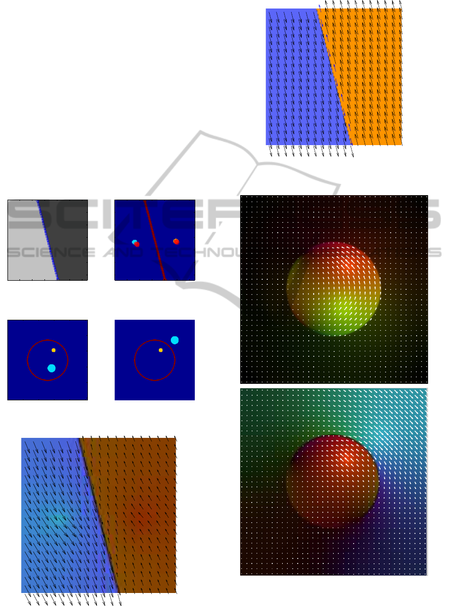
Figure 3: The setup for the planar surface experiments.
Setup of circular experiment: Inside
50 100 150 200 250
50
100
150
200
250
Setup of circular experiment: Outside
Figure 4: The setup for the circular surface experiments.
Figure 5: Results for the planar surface experiment with
objects.
Figure 6: Results for the planar surface experiment with no
objects, but known motion close to the border.
Figure 7: Results for the circular surface experiments. A
color image with overlayed quiver shows the resulting vec-
tor field.
MotionFieldRegularizationforSlidingObjectsUsingGlobalLinearOptimization
321
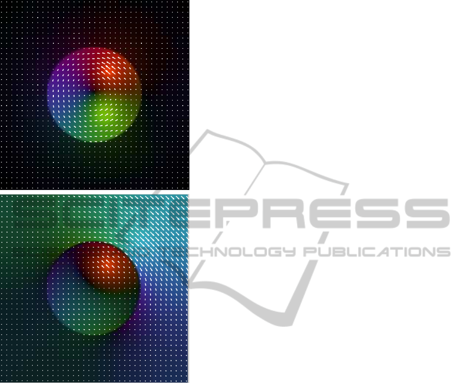
Figure 8: Results for the fixed inner circle.
4 CONCLUSIONS
We have demonstrated a method to perform regular-
ization which allows for areas without friction in the
regularized field. The method has been demonstrated
on six relevant test-cases in 2 dimensions. The meth-
ods are shown to work well even if the vast major-
ity of the data is missing. We also demonstrate that
the GLO framework used is very powerful and allows
for several more simultaneous constraints on different
subsets of the data. One of which is known transla-
tional motion ( known center-of-mass ), which is in-
corporated into two of the test cases. This information
of how to adapt the processing could be incorporated
from for instance medical atlases with a segmentation
done beforehand.
The work is inspired by the method used in (Pace
et al., 2011), but our method uses a tensor instead
of a vector for the orientations normal to the sliding
surface, which allows to treat more complex neigh-
bourhoods - something that would be especially use-
ful for 3D processing. Also the framework in which
our method was implemented allows to combine with
many other models and behaviours for the data pro-
cessing - including non-local constraints such as the
mass-center constraint demonstrated, which is an es-
pecially good property when considering biomedical
image processing, where it would be beneficial to si-
multaneously consider many different physiological
constraints in order to increase the chance of a correct
diagnosis or a successful medical treatment.
5 DISCUSSION
On coarse scales in 3D - for instance cylinders, tubu-
lar structures and edges of cuboids, rank(T) = 2
and therefore rank(P) = 1. This is not possible if
finding an
ˆ
n to the closest boundary and computing
P = (I − w
ˆ
n
ˆ
n
T
) as in (Pace et al., 2011).
Despite the conceputal advantages compared to pre-
viously mentioned method, important future work re-
mains to be done for the proposed method:
1. Tests where noise is present in d.
2. Test cases where noise is present in T.
3. Testing for real clinical data.
4. Implementation in 3 dimensions.
Other important future work includes demonstrat-
ing combining the proposed method with simultane-
ously performing the regularization done in (Johans-
son et al., 2012) and to implement and incorporate
GLO functionality similar to that which is described
in (Ruan et al., 2009). If all of those types of regu-
larization could be combined it would hopefully give
a very powerful platform for global regularization
in medical image registration. Very recently, while
this work was being done, two new registration algo-
rithms which handle sliding of objects were published
(Lianghao et al., 2014) and (Berendsen et al., 2014).
It is difficult for our proposed regularization method
to directly compare to theirs partly because of con-
ceptual differences but mostly because they present
entire registration methods and not only methods for
regularization of missing or uncertain data.
ACKNOWLEDGEMENTS
We would like to thank the Swedish Research Coun-
cil, grant 2011-5176 for project: Dynamic Context
ICPRAM2015-InternationalConferenceonPatternRecognitionApplicationsandMethods
322

Atlases for Image Denoising and Patient Safety and
CADICS - a Linnaeus Research Environment for
funding this research.
REFERENCES
Berendsen, F. F., Kotte, A. N. T. J., Viergever, M. A., and
Pluim, J. P. W. (2014). Registration of organs with
sliding interfaces and changing topologies. In Proc.
SPIE 9034, Medical Imaging 2014: Image Process-
ing, 90340E.
Horn, R. A. and Johnson, C. R. (1990). Matrix Analysis.
Cambridge University Press.
Johansson, G., Forsberg, D., and Knutsson, H. (2012).
Globally optimal displacement fields using local ten-
sor metric. In Proceedings of the International Con-
ference on Image Processing (ICIP).
Lianghao, H., Hawkes, D., and Barrat, D. (2014). A hy-
brid biomechanical model-based image registration
method for sliding objects. In Proc. SPIE 9034, Med-
ical Imaging 2014: Image Processing, 90340G.
Pace, D., Enquobahrie, A., Yang, H., Aylward, S., and Ni-
ethammer, M. (2011). Deformable image registration
of sliding organs using anisotropic diffusive regular-
ization. In Biomedical Imaging: From Nano to Macro,
2011 IEEE International Symposium on, pages 407–
413.
Ruan, D., Esedoglu, S., and Fessler, J. (2009). Discrimina-
tive sliding preserving regularization in medical im-
age registration. In Biomedical Imaging: From Nano
to Macro, 2009. ISBI ’09. IEEE International Sympo-
sium on, pages 430–433.
APPENDIX
For clarification we here write down explicit expres-
sions for some of the terms in the GLO. Assume
matrices have elements denoted as in:
A =
a
11
a
12
·· · a
1N
a
21
a
22
·· · a
2N
.
.
.
.
.
.
.
.
.
.
.
.
a
M1
a
M2
·· · a
MN
(A.10)
A Kronecker product ⊗ between two matrices A and
B is:
A ⊗ B =
a
11
B a
12
B ·· · a
1N
B
a
21
B a
22
B ·· · a
2N
B
.
.
.
.
.
.
.
.
.
.
.
.
a
M1
B a
M2
B ··· a
MN
B
(A.11)
So in our case for 2D, I
2
and the P tensor are:
I
2
=
1 0
0 1
P =
P
11
P
12
P
12
P
22
(A.12)
And then the kronecker product to work on each of
the spatial gradient becomes:
(I
2
⊗ P) =
P
11
P
12
0 0
P
12
P
22
0 0
0 0 P
11
P
12
0 0 P
12
P
22
(A.13)
For ∇ = I
2
⊗ ∇
s
, we get for 2D:
1 0
0 1
⊗
∂
∂x
∂
∂y
!
=
∂
∂x
0
∂
∂y
0
0
∂
∂x
0
∂
∂y
(A.14)
MotionFieldRegularizationforSlidingObjectsUsingGlobalLinearOptimization
323
