
PCB Recognition using Local Features for Recycling Purposes
Christopher Pramerdorfer and Martin Kampel
Computer Vision Lab, Vienna University of Technology, Favoritenstr. 9/183-2, Vienna, Austria
Keywords:
Interest Points, Descriptors, Local Features, Instance Recognition, PCB Recognition, Evaluation.
Abstract:
We present a method for detecting and classifying Printed Circuit Boards (PCBs) in waste streams for recycling
purposes. Our method employs local feature matching and geometric verification to achieve a high open-set
recognition performance under practical conditions. In order to assess the suitability of different local features
in this context, we perform a comprehensive evaluation of established (SIFT, SURF) and recent (ORB, BRISK,
FREAK, AKAZE) keypoint detectors and descriptors in terms of established performance measures. The
results show that SIFT and SURF are outperformed by recent alternatives, and that most descriptors benefit
from color information in the form of opponent color space. The presented method achieves a recognition rate
of up to 100% and is robust with respect to PCB damage, as verified using a comprehensive public dataset.
1 INTRODUCTION
Chemical elements such as gallium, indium, and rare-
earth elements are required for the production of elec-
tronics like integrated circuits, photovoltaics, and flat
panel displays (Moss et al., 2011). In recent years the
demand for these elements has been rising faster than
the supply, and, for certain elements, has already sur-
passed it (Moss et al., 2011). Increasing the produc-
tion capacity is not possible without limitations due
to the geographical concentration of the supply and
trade restrictions, for example (Moss et al., 2011).
For this reason, reclaiming these chemical elements
via recycling is important in order to overcome sup-
ply bottlenecks and to assure a sustainable production
of electronics that demand these elements.
This paper focuses on the optical recognition of
Printed Circuit Boards (PCBs) in waste streams for
recycling purposes. PCBs are a common electronics
waste and, depending on the mounted components,
contain gallium and other valuable elements (Moss
et al., 2011). The purpose of PCB recognition in
waste streams is to detect and classify specific PCBs
that are known to contain such elements, which are
then separated and recycled individually depending
on the particular type. This corresponds to an open-
set instance recognition problem; the task is to detect
and classify known target objects reliably while re-
jecting unknown objects.
To the knowledge of the authors, optical PCB
recognition in waste streams for recycling purposes
is an application that has not been explored so far. A
related application is the optical inspection of PCBs in
order to detect manufacturing defects (Moganti et al.,
1996; Guerra and Villalobos, 2001). Methods for de-
tecting individual PCB components (surface-mounted
devices, through-hole components) for recycling pur-
poses are presented in (Herchenbach et al., 2013; Li
et al., 2013). (Koch et al., 2013) describe a method for
generating 3D models of PCBs via laser triangulation.
These methods operate at the component level
rather than the PCB level or, in case of (Koch et al.,
2013), are designed for PCBs in general. In conse-
quence, they are inadequate for use in recycling sys-
tems that process specific PCBs as a whole.
To this end, we present a method for detecting and
classifying PCBs in waste streams via image analy-
sis.
1
Our method is designed for use in a specific
recycling appliance, which is detailed in Section 2.
This entails distinctive operating conditions, namely
(i) target objects with a characteristic and similar ap-
pearance, (ii) constant illumination, motion blur, and
image noise, and (iii) the absence of significant cam-
era viewpoint changes apart from in-plane rotation. In
order to cope with these conditions, our method em-
ploys object representations based on local features
(local image descriptors computed at interest point lo-
1
This work is supported by the European Union under
grant FP7-NMP (Project reference: 309620). However, this
paper reflects only the authors’ views and the European
Community is not liable for any use that may be made of
the information contained herein.
71
Pramerdorfer C. and Kampel M..
PCB Recognition using Local Features for Recycling Purposes.
DOI: 10.5220/0005289200710078
In Proceedings of the 10th International Conference on Computer Vision Theory and Applications (VISAPP-2015), pages 71-78
ISBN: 978-989-758-091-8
Copyright
c
2015 SCITEPRESS (Science and Technology Publications, Lda.)
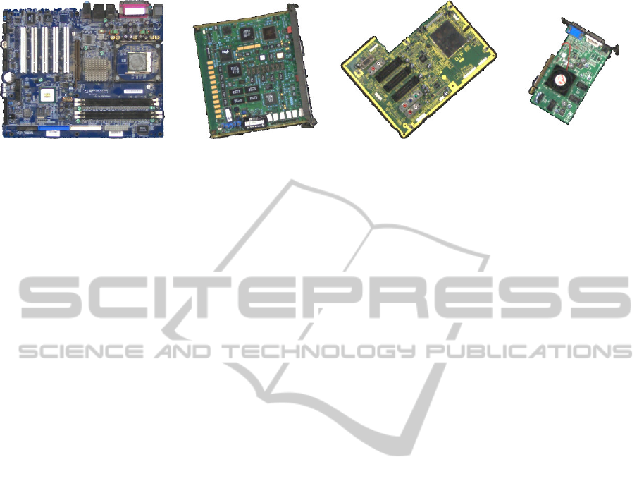
Figure 1: Reference frames obtained via preprocessing.
cations) that are invariant to in-plane rotation and ro-
bust to small perspective distortions and image noise.
Another advantage of such representations is that they
are stable with respect to dust and partially damaged
or broken PCBs due to their part-based nature.
Following the success of SIFT (Lowe, 1999), sev-
eral local feature extractors with different characteris-
tics have been proposed. In order to be able to select
a suitable feature extractor for a given task, the per-
formance characteristics of the different alternatives
must be known. To this end, performance evaluations
of keypoint detectors and descriptor extractors have
been carried out. (Mikolajczyk et al., 2005) presented
a standard dataset for this purpose, the so-called Ox-
ford dataset, and used it to compare affine region de-
tectors. (Mikolajczyk and Schmid, 2005) utilize this
dataset to compare descriptors. (Moreels and Perona,
2007) and (Aanæs et al., 2012) evaluate different key-
points and descriptors on nonplanar objects. (Heinly
et al., 2012) compare different combinations of recent
keypoint detectors and descriptor extractors on two
datasets, including the Oxford dataset.
While the datasets used in these evaluations cover
a broad range of photometric and geometric image
transformations, they do not correspond to the afore-
mentioned operating conditions. For instance, the
Oxford dataset does not contain test cases for motion
blur and pure in-plane rotation. On the other hand, it
does include test cases that do not occur in the con-
text of our application, such as significant viewpoint
and lighting changes. Furthermore, the appearance
characteristics of the depicted objects differ; the test
datasets contain natural scenes and different kinds of
objects, whereas PCBs all have a distinctive, struc-
tured appearance due their component-based compo-
sition (Figure 1). For these reasons, the results re-
ported in these evaluations are inadequate for assess-
ing the suitability of different local features in the dis-
cussed PCB recognition context.
A general limitation of these evaluations is that
they do not cover recent developments such as
FREAK and AKAZE, and that they do not study the
effect of utilizing color information despite the posi-
tive results with SIFT (Van De Sande et al., 2010).
For these reasons, we carry out a comprehensive
evaluation of local features in a PCB recognition con-
text in terms of established performance measures.
The results show that recent binary features outper-
form the established features SIFT and SURF, and
that most features benefit from utilizing color infor-
mation in the form of opponent color space. On this
basis, we select ORB features for PCB recognition,
and show that our method achieves a recognition rate
of up to 100% while being robust to PCB damage.
This paper is organized as follows. Section 2 de-
scribes the PCB recognition setup and our recognition
method. Section 3 discusses different local feature ex-
tractors, details the evaluation protocol, and presents
the evaluation results. The recognition performance
of our method is analyzed in Section 4. Conclusions
are drawn in Section 5.
2 PCB RECOGNITION
The proposed recognition method is used in an appli-
ance for recognizing specific PCBs in waste streams
in real-time. As such, the input is a live stream from
an IP camera (1280x960 px resolution, approx. 50
pixels per inch) . The appliance includes a black
conveyor belt that carries the waste stream at a con-
stant velocity of about 0.2 m/s. The camera is located
above the conveyor belt, oriented such that the image
plane and the conveyor belt are parallel to each other.
The appliance provides constant illumination by po-
larized light, which, in conjunction with a polariza-
tion filter in front of the camera, suppresses specular
reflections. Figure 2 illustrates this setup.
PCB recognition is accomplished in two steps.
First, individual objects in the waste stream are de-
tected and tracked over time, in order to be able to
extract a suitable reference image for each object. We
refer to this step as preprocessing. Subsequently, each
reference image is analyzed by means of local feature
matching and geometric verification.
VISAPP2015-InternationalConferenceonComputerVisionTheoryandApplications
72
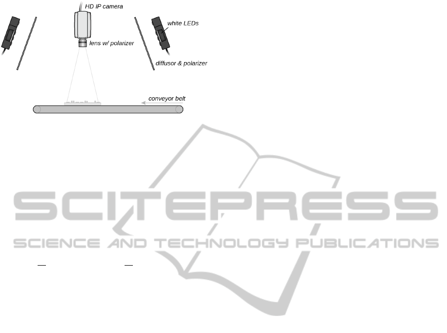
Figure 2: Image acquisition setup.
2.1 Preprocessing
Individual objects are detected via background sub-
traction. We employ a unimodal background model,
which is sufficient considering the stable illumination
and conveyor belt appearance. More precisely, we
model the intensity distribution of the conveyor belt
as a single Gaussian for each pixel and learn the pa-
rameters from M frames during system initialization,
ˆµ
x,y
=
1
M
M
∑
m=1
T
m
x,y
ˆ
σ
2
x,y
=
1
M
(T
m
x,y
− ˆµ
x,y
)
2
. (1)
T
m
x,y
denotes the pixel value at position (x, y) in the
mth frame after smoothing via linear filtering. At run-
time, each pixel of the current frame F
x,y
is classi-
fied as background if F
x,y
− ˆµ
x,y
< 3
ˆ
σ
x,y
, otherwise as
foreground. Afterwards, small holes and noise are re-
moved via morphological closing and opening.
The resulting binary foreground mask is subject to
connected component analysis. Components whose
size (number of pixels) is too small to represent PCBs
are discarded. The remaining components are tracked
over time on a frame-by-frame basis, with each com-
ponent being represented by its centroid location. The
goal is thus to find, in each frame, the optimal asso-
ciation between C components and T tracks. We for-
mulate this task as an energy minimization problem,
with the energy between a component and a track be-
ing the Euclidean distance between the correspond-
ing centroid locations. Track centroid locations are
estimated from previous observations via Kalman fil-
tering (Kalman, 1960). We ensure that C = T by in-
troducing dummy tracks and components if required
(Papadimitriou and Steiglitz, 1982), which enables us
to find the optimal association efficiently using the
Hungarian algorithm (Kuhn, 1955).
The tracking information allows us to select a suit-
able reference frame for each observed PCB candi-
date; we select the frame in which the distance be-
tween the camera principal point and the component
centroid location is minimal. This ensures a similar
viewpoint between observed PCB images and mini-
mizes perspective distortions. Figure 1 shows refer-
ence frames obtained this way. After correcting for
lens distortions, each reference image is processed in
an open-set recognition context.
2.2 PCB Recognition
PCBs are recognized by extracting local features from
the input reference image, which are then matched
to the features of each PCB that should be recog-
nized. These features are stored in a database together
with metadata that facilitate recycling. Features are
matched using the descriptor distance ratio test pro-
posed in (Lowe, 2004).
A key characteristic of our recognition method is
that it utilizes the fact that PCBs are flat and that the
camera position is stable to perform geometric veri-
fication; the feature matches are used to estimate the
homography H that describes the mapping between
both feature sets. RANSAC is used for robustness
with respect to erroneous matches, and all matches
that do not agree with H are discarded (a match agrees
with H if both feature locations are close under H).
The number of agreeing matches is used as the sim-
ilarity measure. Furthermore, H is tested for plausi-
bility; due to the preprocessing step, two images of
the same PCB are, in approximation, related by an in-
plane rotation, which implies det(H) ≈ 1. If this is
not the case, a similarity of 0 is assumed.
On this basis, recognition is performed by clas-
sifying the input image as the PCB with the highest
similarity. This applies unless this similarity is below
a threshold, in which case the image is rejected.
We do not employ techniques used in large-scale
image recognition such as bag of words (Sivic and
Zisserman, 2003). Our recognition method is used
with small databases (less than 100 PCBs), which, in
conjunction with features that can be matched effi-
ciently, ensures real-time analysis. By not resorting
to these techniques, we avoid the associated perfor-
mance decrease due to the incurred information loss.
3 FEATURE EVALUATION
Our PCB recognition method supports arbitrary local
features. To obtain information on the performance
characteristics of different features in the discussed
context, we compare different candidates in terms of
precision vs. recall and descriptor matching score,
two established performance measures. To study the
effect of color information, this comparison is carried
out on grayscale images as well as in opponent color
PCBRecognitionusingLocalFeaturesforRecyclingPurposes
73

Table 1: Key characteristics of the analyzed keypoint-descriptor pairings (II: intensity invariance, RI: rotation invariance, SI:
scale invariance, AI: affine invariance, ES: feature extraction speed, MS: feature matching speed, BD: binary descriptor, DS:
descriptor size). Speed rankings are based on (Heinly et al., 2012; Alcantarilla et al., 2013; Alahi et al., 2012).
Keypoints Descriptors Reference II RI SI AI ES MS BD DS
SIFT SIFT (Lowe, 2004) Y Y Y N 6 5 N 128 Bytes
SURF SURF (Bay et al., 2006) Y Y Y N 5 4 N 64 Floats
SURF FREAK (Alahi et al., 2012) Y Y Y N 4 3 Y 512 Bits
ORB ORB (Rublee et al., 2011) Y Y Y N 1 1 Y 256 Bits
BRISK BRISK (Leutenegger et al., 2011) Y Y Y N 2 3 Y 512 Bits
AKAZE AKAZE (Alcantarilla et al., 2013) Y Y Y N 3 2 Y 488 Bits
space. Table 1 summarizes the analyzed features re-
spectively keypoint-descriptor pairings and their key
characteristics. For brevity, we henceforth refer to
these features by their descriptor names (e.g. FREAK
instead of SURF-FREAK).
All features are tested with default parameters as
stated in the corresponding publications, with the ex-
ception of keypoint detector thresholds. These thresh-
olds are selected such as to limit the number of de-
tected keypoints to 500 in order to mitigate the effect
of the number of keypoints on performance scores
(Mikolajczyk et al., 2005). The Euclidean and Ham-
ming distance is used for matching real and binary
descriptors, respectively. We use OpenCV (version
2.4.9) implementations of all features except BRISK
and AKAZE. For BRISK we resort to the code pro-
vided by the author (Leutenegger et al., 2011) due to
a performance-degrading bug in recent OpenCV ver-
sions. As AKAZE is not part of OpenCV at the time
of writing, we use the implementation provided by the
authors (Alcantarilla et al., 2013), adapted to support
opponent color space.
For evaluation we employ a dataset consisting of
six reference images for each of 25 PCBs in ran-
dom orientations, obtained as discussed in Section
2.1. As such, the dataset tests the feature perfor-
mance in presence of constant illumination, motion
blur, image noise, and with a focus on in-plane ro-
tation. The depicted PCBs originate from a waste
stream in a recycling facility. The dataset is thus rep-
resentative in terms of both the depicted PCBs and
their condition (e.g. dust and damages). Figure 1
shows example images. The dataset is publicly avail-
able at http://www.caa.tuwien.ac.at/cvl/research/pcb-
ip-dataset/index.html. We manually annotate key-
points in all images (only points on the boards them-
selves, not on mounted components). For each PCB,
we select one image as the reference and use the anno-
tations to compute ground-truth homographies to the
remaing images.
We note that the test PCBs are not perfectly pla-
nar. As such, the relation between images of the same
PCB cannot be precisely described by a homography
over the whole domain. While this circumstance im-
pacts established performance measures that depend
on ground-truth homographies, it affects all tested
features alike and thus does not favor certain features.
3.1 Precision vs. Recall
Precision and recall are established performance mea-
sures that encode the number of correct and incor-
rect feature matches between two images. We calcu-
late these measures as in (Mikolajczyk and Schmid,
2005). Two features are matches if the distance be-
tween their descriptors is below t
d
. If the region over-
lap between the corresponding keypoints (the ratio
between the intersection and the union of their regions
after scale normalization) after applying the ground-
truth homography is larger than t
r
= 0.5, the match
is deemed correct. On this basis, the precision is
calculated as the share of correct matches among all
matches. The recall is the fraction between the num-
ber of correct matches and the number of keypoint
correspondences in terms of region overlap. We vary
t
d
to generate 1−precision vs. recall graphs. The re-
ported values are averages over all images.
As shown in Figure 3, FREAK performs best over
the whole precision range, with AKAZE being ranked
second. Both features have a clear performance ad-
vantage over the competitors in the high-precision
range. SIFT performs worst because it extracts sev-
eral descriptors per keypoint if multiple dominant
keypoint orientations are found, which impacts the re-
call (Leutenegger et al., 2011).
All features except SURF and AKAZE benefit
from opponent color space (Figure 4). FREAK,
which again performs best over the whole domain,
improves by 5-10% on average. BRISK benefits the
most from opponent color space, with gains between
10% and 15%. SIFT shows moderate performance
gains in the high-precision range, whereas the perfor-
mance of AKAZE decreases significantly.
VISAPP2015-InternationalConferenceonComputerVisionTheoryandApplications
74
●
●
●
●
●
●
●
●
●
●
●
0.00
0.25
0.50
0.75
1.00
0.00 0.25 0.50 0.75 1.00
1 − Precision
Recall
Method
●
AKAZE−AKAZE
BRISK−BRISK
ORB−ORB
SIFT−SIFT
SURF−FREAK
SURF−SURF
Figure 3: 1−Precision vs. recall (grayscale images).
●
●
●
●
●
●
●
●
●
●
0.00
0.25
0.50
0.75
1.00
0.00 0.25 0.50 0.75 1.00
1 − Precision
Recall
Method
●
AKAZE−AKAZE
BRISK−BRISK
ORB−ORB
SIFT−SIFT
SURF−FREAK
SURF−SURF
Figure 4: 1−Precision vs. recall (opponent color space).
3.2 Descriptor Matching Score
A common strategy for matching features between
two images is the descriptor distance ratio test, which
matches two features f
i
, f
j
if f
j
is the nearest neigh-
bor of f
i
in terms of descriptor distance and if the dis-
tance ratio between f
i
and the first and second near-
est neighbors, respectively, is below t
f
= 0.8 (Lowe,
2004). This strategy effectively suppresses incorrect
matches while preserving correct matches. In order
to evaluate the feature performance in this regard, we
use this strategy to obtain matches between all image
pairs, and compute the descriptor matching score as
the fraction of matches that agree with the ground-
truth homography ((Heinly et al., 2012) refer to this
measure as the precision). A match is in agreement if
the corresponding keypoint locations are within t
k
= 5
pixels distance from each other after applying the
ground-truth homography. We set t
k
comparatively
large (a common value in the literature appears to be
t
k
= 2.5) to compensate for the fact that the test ob-
jects are not perfectly planar. The reported values are
again averages over all images.
Figure 5 illustrates that all binary features exhibit
similar matching scores on grayscale images, and that
these scores are 7-10% higher than those of SIFT and
SURF. AKAZE performs best in this experiment as it
yields the largest number of correct matches, followed
by FREAK and ORB. BRISK achieves the high-
est matching score, which is consistent with (Heinly
et al., 2012), but returns the lowest number of correct
matches among all binary features. The results also
show a large variation in the number of matches and
the matching score due to the differences in test object
appearance. BRISK is most stable in this regard.
●
0.6
0.7
0.8
0.9
1.0
100 150 200 250 300
Matches
Matching Score
Method
●
AKAZE−AKAZE
BRISK−BRISK
ORB−ORB
SIFT−SIFT
SURF−FREAK
SURF−SURF
Figure 5: Average number of matches and matching scores
(grayscale images). Bars mark ±1 standard deviations.
Utilizing opponent color space improves the
matching score by 3-5% (Figure 6). The exception
is SIFT with an improvement of 10%, which renders
it competitive to the binary features. The winner in
terms of matching score is again BRISK. Opponent
color space decreases the number of matches in all
cases, with ORB, FREAK, and BRISK being the most
stable in this regard. AKAZE again returns the largest
number of correct matches, followed by FREAK and
ORB. SURF performs worse than the competitors.
3.3 Discussion and Feature Selection
The feature evaluation results show that the estab-
lished features SIFT and SURF are outperformed by
more recent alternatives with binary descriptors in
most experiments. The performance ranking depends
on the feature matching strategy; FREAK achieves
better results than the competition with threshold-
based matching, whereas AKAZE performs best in
case of distance-ratio-based matching.
As the results are obtained from a dataset with dis-
tinctive characteristics (Section 1), they agree with the
PCBRecognitionusingLocalFeaturesforRecyclingPurposes
75

●
0.6
0.7
0.8
0.9
1.0
100 150 200 250 300
Matches
Matching Score
Method
●
AKAZE−AKAZE
BRISK−BRISK
ORB−ORB
SIFT−SIFT
SURF−FREAK
SURF−SURF
Figure 6: Average number of matches and matching scores
(opponent color space). Bars mark ±1 standard deviations.
literature only partially. For example, (Alahi et al.,
2012) also find that FREAK outperforms BRISK,
SIFT, and SURF with threshold-based matching, but
the ranking differs. SIFT is reported to perform fa-
vorably to both BRISK, ORB, and SURF under pure
in-plane rotations both in terms of precision vs. re-
call and descriptor matching score (Leutenegger et al.,
2011; Heinly et al., 2012), which contrasts to our find-
ings. As discussed in Section 1, this is attributed to
the different appearance characteristics of the test ob-
jects. The disagreement between previous and our re-
sults highlights the importance of feature evaluations
that accurately capture the operating conditions.
Furthermore, the results show that most descrip-
tors, particularly FREAK, BRISK, ORB, and SIFT,
benefit from opponent color space, which was origi-
nally conceived for SIFT (Van De Sande et al., 2010).
We therefore put forward to use opponent color space
with all these descriptors if a high matching perfor-
mance is paramount, unless the computational over-
head is a limiting factor; employing opponent color
space instead of grayscale images increases the fea-
ture extraction complexity and descriptor size by a
factor of 3. The performance of AKAZE regresses in
opponent color space with threshold-based matching.
We will investigate this issue in the future.
On the basis of these results, we select ORB fea-
tures for use with our recognition method. These fea-
tures achieve a competitive performance in all exper-
iments while being the most efficient to compute and
match (Table 1). Computing 500 ORB features in a
test image takes around 18ms on a PC with an Intel i7
CPU, and feature matching takes only about 7ms.
4 EXPERIMENTAL RESULTS
We assess the performance of the proposed PCB
recognition method using a dataset consisting of 480
PCB images (six images for each of 80 PCBs). The
PCBs originate from a recycling facility and the im-
ages were obtained as described in Section 3.
For evaluation purposes, we randomly select 25
images of different PCBs for the database and pro-
cess the 455 remaining images as described in Section
2.2 (matches are rejected if | det(H) − 1| > 0.5). We
use ORB features and compare results obtained using
grayscale images to those using opponent color space.
In practice, waste PCBs are often partially dam-
aged or broken. In order to investigate the robust-
ness with respect to broken PCBs, we set a fraction
of z PCB pixels to zero before applying our recog-
nition method to simulate missing PCB pieces. This
is accomplished on a per-row basis to ensure that the
missing fraction constitutes a contiguous area; we it-
eratively set consecutive image rows to zero until the
number of visible PCB pixels decreases below 1 − z
times the original number. We repeat the test de-
scribed above for z = {0, 0.1, 0.2, . . . , 0.9}.
For each z, we calculate the the overall error rate
(ERR) as the fraction of images that are classified cor-
rectly, regardless of whether the depicted PCBs exist
in the database. Furthermore, we compute the false
classification rate (FCR) as the fraction of images that
are represented in the database but assigned to an in-
correct class, the false rejection rate (FRR) as the frac-
tion of images that are rejected even though they are
represented in the database, and the false accept rate
(FAR) as the fraction of images that are classified as
in the database even tough this is not the case.
Figure 7 summarizes the experimental results.
With z = 0 (i.e. with intact PCBs), no errors are ob-
served; all target PCBs are recognized correctly and
all other PCBs are rejected. Increasing z increases
only the FRR (which in turn affects the ERR); both
the FCR and FAR remain zero in all tests. With
z = 0.2 and z = 0.5 (i.e. with 20% respectively 50%
missing data), the FRR is 3% and 19%, respectively.
The results obtained using grayscale images are al-
most identical to those obtained using opponent color
space over the whole domain of z.
The results confirm the suitability of the proposed
method for PCB recognition in a recycling context.
The method achieves a recognition rate of 100% with
intact PCBs and is robust with respect to broken
PCBs; even with 50% missing data (which corre-
sponds to a PCB that was broken in half), 80% of
target PCBs are detected and classified correctly. Due
to homography verification, the method is remarkably
VISAPP2015-InternationalConferenceonComputerVisionTheoryandApplications
76
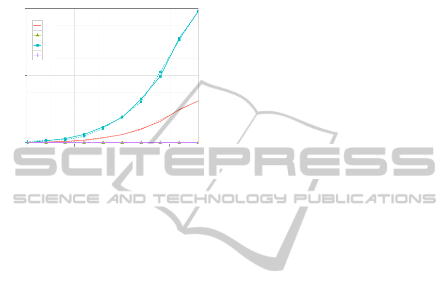
robust in terms of classification errors; both the FCR
and FAR are zero even with 90% missing data. This
is important in the discussed context as it ensures that
selective recycling lines are not contaminated.
●
●
●
●
●
●
●
●
●
●
●
●
●
●
●
●
●
●
●
●
0
25
50
75
100
0.00 0.25 0.50 0.75
Fraction of Missing Data
Error Percentage
Score
●
ERR
FCR
FRR
FAR
Figure 7: Recognition performance of the proposed
method, using ORB features. Continuous lines denote re-
sults obtained using grayscale images, while dashed lines
represent results obtained using opponent color space.
5 CONCLUSIONS
We have presented a method for recognizing specific
PCBs in waste streams via local feature matching and
geometric verification. The method achieves an open-
set recognition rate of up to 100% on a comprehen-
sive test dataset while being robust with respect to
broken PCBs. It is a key component in a recycling
appliance designed for reclaiming valuable chemical
elements and thus contributes to overcoming supply
bottlenecks and to sustainable electronics production.
Furthermore, we have performed a comprehen-
sive evaluation of local features in a new applica-
tion context, namely with respect to PCB recogni-
tion. The evaluation results show that ORB, BRISK,
FREAK, and AKAZE outperform SIFT and SURF
in this context. The differences between our find-
ings and previous results highlight the need for task-
specific test datasets. We contribute to the body of
available datasets by providing an extensive, freely
available dataset consisting of PCB images.
Moreover, we have demonstrated that utilizing
color information in the form of opponent color space
is beneficial not only to SIFT, but also to ORB,
BRISK, and FREAK.
REFERENCES
Aanæs, H., Dahl, A. L., and Pedersen, K. S. (2012). Inter-
esting interest points. International Journal of Com-
puter Vision, 97(1):18–35.
Alahi, A., Ortiz, R., and Vandergheynst, P. (2012). FREAK:
Fast Retina Keypoint. In IEEE Conference on Com-
puter Vision and Pattern Recognition, pages 510–517.
Alcantarilla, P. F., Nuevo, J., and Bartoli, A. (2013). Fast
Explicit Diffusion for Accelerated Features in Non-
linear Scale Spaces. In British Machine Vision Con-
ference, pages 13.1–13.11.
Bay, H., Tuytelaars, T., and Van Gool, L. (2006). SURF:
Speeded up robust features. In European Conference
on Computer Vision, pages 404–417. Springer.
Guerra, E. and Villalobos, J. (2001). A three-dimensional
automated visual inspection system for SMT assem-
bly. Computers & industrial engineering, 40(1):175–
190.
Heinly, J., Dunn, E., and Frahm, J.-M. (2012). Comparative
evaluation of binary features. In European Conference
on Computer Vision, pages 759–773. Springer.
Herchenbach, D., Li, W., and Breier, M. (2013). Segmen-
tation and classification of THCs on PCBAs. In IEEE
International Conference on Industrial Informatics,
pages 59–64.
Kalman, R. E. (1960). A New Approach to Linear Filtering
and Prediction Problems. Transactions of the ASME–
Journal of Basic Engineering, 82(D):35–45.
Koch, T., Breier, M., and Li, W. (2013). Heightmap genera-
tion for printed circuit boards (PCB) using laser trian-
gulation for pre-processing optimization in industrial
recycling applications. In IEEE International Confer-
ence on Industrial Informatics, pages 48–53.
Kuhn, H. W. (1955). The Hungarian method for the assign-
ment problem. Naval Research Logistics Quarterly,
2(1):83–97.
Leutenegger, S., Chli, M., and Siegwart, R. Y. (2011).
BRISK: Binary robust invariant scalable keypoints. In
IEEE International Conference on Computer Vision,
pages 2548–2555.
Li, W., Esders, B., and Breier, M. (2013). SMD segmen-
tation for automated PCB recycling. In IEEE Inter-
national Conference on Industrial Informatics, pages
65–70.
Lowe, D. G. (1999). Object recognition from local scale-
invariant features. In IEEE International Conference
on Computer Vision, volume 2, pages 1150–1157.
Lowe, D. G. (2004). Distinctive image features from scale-
invariant keypoints. International Journal of Com-
puter Vision, 60(2):91–110.
Mikolajczyk, K. and Schmid, C. (2005). A perfor-
mance evaluation of local descriptors. IEEE Trans-
actions on Pattern Analysis and Machine Intelligence,
27(10):1615–1630.
Mikolajczyk, K., Tuytelaars, T., Schmid, C., Zisserman, A.,
Matas, J., Schaffalitzky, F., Kadir, T., and Van Gool, L.
(2005). A comparison of affine region detectors. Inter-
national Journal of Computer Vision, 65(1-2):43–72.
PCBRecognitionusingLocalFeaturesforRecyclingPurposes
77

Moganti, M., Ercal, F., Dagli, C. H., and Tsunekawa, S.
(1996). Automatic PCB inspection algorithms: a
survey. Computer vision and image understanding,
63(2):287–313.
Moreels, P. and Perona, P. (2007). Evaluation of features
detectors and descriptors based on 3d objects. Inter-
national Journal of Computer Vision, 73(3):263–284.
Moss, R., Tzimas, E., Kara, H., Willis, P., and Kooroshy, J.
(2011). Critical Metals in Strategic Energy Technolo-
gies. JRC-scientific and strategic reports.
Papadimitriou, C. and Steiglitz, K. (1982). Combinatorial
Optimization: Algorithm and Complexity. Prentice
Hall.
Rublee, E., Rabaud, V., Konolige, K., and Bradski, G.
(2011). ORB: an efficient alternative to SIFT or
SURF. In IEEE International Conference on Com-
puter Vision, pages 2564–2571.
Sivic, J. and Zisserman, A. (2003). Video Google: A text
retrieval approach to object matching in videos. In
IEEE International Conference on Computer Vision,
pages 1470–1477.
Van De Sande, K. E., Gevers, T., and Snoek, C. G. (2010).
Evaluating color descriptors for object and scene
recognition. IEEE Transactions on Pattern Analysis
and Machine Intelligence, 32(9):1582–1596.
VISAPP2015-InternationalConferenceonComputerVisionTheoryandApplications
78
