A Particle-based Dissolution Model using Chemical Collision Energy

Min Jiang, Richard Southern and Jian Jun Zhang

National Centre for Computer Animation, Bournemouth University, Bournemouth, U.K.

Keywords:

Dissolution, Solute, Solvent, Collision Theory, Activation Energy, Particle Excitation, SPH, Erosion.

Abstract:

We propose a new energy-based method for real-time dissolution simulation. A uniﬁed particle representation

is used for both ﬂuid solvent and solid solute. We derive a novel dissolution model from the collision theory

in chemical reactions: physical laws govern the local excitation of solid particles based on the relative motion

of the ﬂuid and solid. When the local excitation energy exceeds a user speciﬁed threshold (activation energy),

the particle will be dislodged from the solid. Unlike previous methods, our model ensures that the dissolution

result is independent of solute sampling resolution. We also establish a mathematical relationship between

the activation energy, the inter-facial surface area, and the total dissolution time — allowing for accurate

artistic control over the global dissolution rate while maintaining the physical plausibility of the simulation.

We demonstrate applications of our method using a number of practical examples, including antacid pills

dissolving in water and hydraulic erosion of non-homogeneous terrains. Our method is straightforward to

incorporate with existing particle-based ﬂuid simulations.

1 INTRODUCTION

The reliance of ﬁlms and games on realistic ﬂuid

simulations has led to the popularity of this research

topic, with most work in this ﬁeld focused on the

behaviour of ﬂuid itself, such as spray, waves and

bubbles (Ihmsen et al., 2012; Cleary et al., 2007;

Busaryev et al., 2012) or the interaction with solids

(Batty et al., 2007; Robinson-Mosher et al., 2008;

Schechter and Bridson, 2012; Akinci et al., 2013).

Comparatively few researchers have tackled the chal-

lenging problem of the chemical reaction between

ﬂuid and solids, which, under the right conditions, can

lead to solid mixing with the liquid: a phenomenon

known as dissolution. The solid in this case is called

the solute and the liquid is the solvent.

Our paper proposes an energy–based dissolution

model to describe this complicated ﬂuid–solid inter-

action. Dissolution is the result of physical and chem-

ical processes: our dissolution model follows colli-

sion theory which explains how the chemical reac-

tion happens. We introduce a kinetic energy func-

tion to measure the particle excitation of the so-

lute, which ensures the same dissolution results even

when the object sampling resolutions are different.

This approach is advantageous when performing pre-

visualization of the phenomena, allowing animators

to quickly preview the dissolution behaviour with a

low resolution sampling of the solute.

A solute particle will become dislodged if the lo-

cal energy exceeds a user speciﬁed activation energy.

While physically justiﬁed, this threshold does not pro-

vide a user with an intuition of the total dissolution

time. We demonstrate that the activation energy can

be approximated as a function of the inter-facial sur-

face area of the solvent/solute and the total dissolution

time, providing animators with a tool to more accu-

rately predict the total dissolution rate.

The key contributions of this paper include:

1. a uniﬁed particle framework which generates

physically and chemically plausible dissolution

behaviour that is simple to incorporate with an

existing particle–based ﬂuid system;

2. an expression for measuring the local particle ex-

citation derived from kinetic energy which is in-

dependent of solute sampling resolution; and

3. a mapping between the global dissolution time

and local particle excitation based on the activa-

tion energy.

Our particle–based method enables real–time perfor-

mances using a parallel implementation. We demon-

strate plausible dissolution behaviours in different cir-

cumstances, such as rotating and translating solids in

ﬂuids and pouring ﬂuids onto dissolving objects. Due

to the similarity between hydraulic erosion and disso-

lution, our dissolution model is able to simulate ero-

sion without any additional computational overhead.

285

Jiang M., Southern R. and Zhang J..

A Particle-based Dissolution Model using Chemical Collision Energy.

DOI: 10.5220/0005290302850293

In Proceedings of the 10th International Conference on Computer Graphics Theory and Applications (GRAPP-2015), pages 285-293

ISBN: 978-989-758-087-1

 2015 SCITEPRESS (Science and Technology Publications, Lda.)

2 RELATED WORK

The simulation of natural phenomena is one of the

most studied areas in Computer Graphics, enabling

animators to generate complex and physically plau-

sible dynamics which would be impossible to create

manually. We only review work related to dissolution

since there is a large body of work in ﬂuid simulation.

In most observable systems, the most frequent sol-

vent is ﬂuid and solute is solid. There have been many

studies on the physical interaction between ﬂuids and

solids. (Arash et al., 2003) studied the ﬂuid–solid

interaction by representing solid with linked point

masses. (Batty et al., 2007) applied a pressure projec-

tion method with kinetic energy minimization to in-

corporate irregular boundary geometry into standard

grid–based ﬂuid simulations. Their methods are yet

difﬁcult to cooperate in dissolution simulation.

(Carlson et al., 2004) and (Amada, 2006) treated

the objects as if they were made of ﬂuid. To main-

tain the object rigidity, (Carlson et al., 2004) identi-

ﬁed the object by velocity ﬁeld, and (Amada, 2006)

applied a corrective step to bring back the rigidity of

the solid. (Harada et al., 2007) simulated the inter-

action using collision detection. To prevent ﬂuid par-

ticles intersecting the solid boundary, both (Amada,

2006) and (Harada et al., 2007) used penalty force

method, which took a few frames to push the particles

out. (Becker et al., 2009) also dealt with boundary

conditions to ensure no–penetration. However, they

required two additional neighbour queries for colli-

sion detection, which was expensive to compute.

(Schechter and Bridson, 2012) achieved the no–

separation and no–slip boundary condition by sam-

pling the air and solid surface as ghost particles. (Ak-

inci et al., 2012) used corrected density to compute

the pressure and viscosity force to avoid the sticking

artefacts. Both solved the boundary problem, mak-

ing an extension to support dissolution simulation. In

this paper we use the similar method with (Akinci

et al., 2012) to handle the boundary problem during

the ﬂuid–solid interaction, but we sample the entire

object rather than just the surface since the boundary

changes as the shape dissolves.

The methods above tackled the problem of physi-

cal interaction between the ﬂuid and solid, but did not

consider the chemical interaction between them. Rel-

atively few attempts have been made to simulate the

complex chemical reaction between ﬂuid and solid.

(Solenthaler et al., 2007) used an elasticity model

for particle–based objects and modelled temperature

for phase changes, allowing them to simulate objects

melting in hot liquid. (Stomakhin et al., 2014) intro-

duced augmented MPM for phase-change and simu-

lated butter melting in pan. Melting offers a simi-

lar visual result with dissolution, but the underlying

function is a heat model, which is different from the

chemical model in this paper.

(Kim et al., 2010) simulated bubbles around dis-

solving objects. Their focus was on simulating the

dispersed bubble ﬂow — the dissolution model was

approximated by generating offsets of a level–set rep-

resentation of the solute, which had little relationship

with actual dissolution behaviour. (Shin et al., 2010)

simulated solids dissolving in liquids by modelling

solid mass transfer. They treated the solvent and so-

lution as different ﬂuids, and used multiple level–sets

to track mixing surfaces which needed to be updated

whenever the reactions and interactions occurred —

an expensive but necessary step. They also didn’t

consider about the object separation during dissolu-

tion. The latter problem is solved in (Wojtan et al.,

2007). However, they both use level–set represen-

tation to guide the object surface without additional

treatment which means their dissolution results will

largely depend on the level-set grid resolution. Fur-

thermore, all these previous approaches did not con-

sider the relationship between the dissolution time

and the mass transfer of the solute, meaning that pre-

dicting the overall dissolution time is an exercise in

trial and error. In this paper we propose a model for

predicting total dissolution time from activation en-

ergy, and our dissolution model is independent of so-

lute sampling resolutions.

Dissolution also shares many properties with hy-

draulic erosion. (Bene

s et al., 2006) proposed a so-

lution for erosion simulation by using Navier–Stokes

equations, while (Wojtan et al., 2007) animated corro-

sion and erosion by driving the ﬂuids with a ﬁnite dif-

ference simulation and presenting the solid by advect-

ing the level sets inward. (Kri

stof et al., 2009) used

an SPH based method to simulate erosion, where the

erosion model is adapted from an Eulerian approach.

The erosion rate used in (Kri

stof et al., 2009; Woj-

tan et al., 2007) is derived from the power law, which

unfortunately requires a large number of parameters

to control, making it impractical for use by an anima-

tor. In this paper we demonstrate two practical ero-

sion examples, including one which demonstrates the

speciﬁcation of non–homogeneous solutes forming a

natural layering stratum.

3 DISSOLUTION MODEL

In the following sections we present a model for

simulating objects dissolving in ﬂuid, derived from

the physics and chemistry behind the solute–solvent

GRAPP2015-InternationalConferenceonComputerGraphicsTheoryandApplications

286

interaction. Collision theory was ﬁrstly proposed

by (Trautz, 1916). It describes how chemical reac-

tions take place and why chemical reaction rates dif-

fer (McNaught and Wilkinson, 1997). Collision the-

ory is closely related to the kinetic-molecular theory:

molecules are in constant motion, occasionally col-

liding as they move. For a chemical reaction to occur,

molecules need to collide in the right orientation and

with sufﬁcient energy (Clark, 2004). The energy re-

quired for the reaction to occur is referred to as the

activation energy — necessary to break the existing

chemical bonds between substrate molecules.

In our system we volumetrically represent both the

solute and the solvent with particles, with each parti-

cle becoming a representative component of the corre-

sponding substance. This uniﬁed particle representa-

tion removes the need for special handling of mixing

surfaces. When solute particles collide with the sol-

vent particles, energy is added to the solute particle.

Each solute particle carries the energy information

which is summed over all the collisions which have

occurred. When the energy is larger than a threshold

energy—the activation energy—the particle detaches

from the object. This activation energy becomes an

important factor in determining the dissolution rate.

This method allows us to model the dissolution pro-

cess in a physically and chemically correct manner.

3.1 Solvent Representation

Most ﬂuid simulation methods are governed by the

Navier–Stokes equations (Foster and Metaxas, 1996).

From the viewpoints of the Lagrangian (particle–

based) and Eulerian (grid–based) methods, particle–

based methods seem to be a natural choice for dis-

solution because it is easy to implement with arbi-

trary boundaries and applied forces, while supporting

ﬂuid mixing and interaction with arbitrary rigid bod-

ies. Smoothed Particle Hydrodynamics (SPH) was

ﬁrst introduced as a mesh–free Lagrangian method in-

dependently by both (Gingold and Monaghan, 1977)

and (Lucy, 1977), and is being increasingly used for

ﬂuid simulation due to its simplicity. In our model,

the physical and chemical reactions between ﬂuid and

solid are elegantly simulated by a single SPH solver.

Our method is implemented within the framework

of SPH model of (M

uller et al., 2003), but is com-

patible with other SPH models (Ihmsen et al., 2014),

such as PCISPH (Solenthaler and Pajarola, 2009), and

can be extended with other particle–based represen-

tations. We demonstrate the basic SPH model with a

short introduction which is required to understand our

dissolution method in the following sections. In SPH,

a scalar quantity A at location x is computed by

A(x) =

∑

W (x − x

, h), (1)

where W (x, h) is a smoothing kernel with smooth

core radius h which also decides the neighbour-

hood size. The kernel satisﬁes

W (x, h)dx = 1 and

W (x, h) = 0 when kxk > h. Particle j is the neigh-

bour of the particle at x. m

is the particle mass and

is the ﬁeld quantity at x

The density and pressure force of the solvent are

calculated also based on (M

uller et al., 2003). Neigh-

bour searching of the solvent simulation is GPU par-

alleled using framework of (Hoetzlein, 2014).

3.2 Solute Representation

The enclosing volume of the solute is sampled by

particles, each of which contributes to the ﬂuid SPH

to ensure the correctness of the ﬂuid–solid interac-

tion: (Akinci et al., 2012) and (Schechter and Brid-

son, 2012) are both good choices for this task. The

pressure between the ﬂuid and solid automatically re-

pels the ﬂuid particles and naturally produces the mix-

ing surface with more accuracy at lower computa-

tional cost than level–set methods. Since we focus on

the dissolution effect when the ﬂuid interacts with the

solid, we need to sample the entire object rather than

boundary particles to produce the volume change.

For the examples used in this paper, a regular grid

sampling is used for the solute. While we have ex-

perimented with alternative sampling techniques, but

these did not alter our results signiﬁcantly and are not

the focus of this paper.

3.2.1 Sampling Independent Dissolution

Our method ensures the same dissolution result

(within error tolerance) even when the sampling res-

olutions of the solute are different. This property

has important applications in computer graphics: for

the purposes of pre–visualisation, the dissolution of

a lower resolution or adaptively sampled object can

be used to predict the behaviour of a very densely

sampled object, or simply to improve performance for

real–time applications.

In previous methods (Wojtan et al., 2007; Shin

et al., 2010) shape alteration of a dissolving object

was achieved using mass transfer. Both methods used

level–sets to represent the solute, causing the dissolu-

tion result to be largely affected by the grid resolution.

In our method we use volume mass instead of mass

for each solute particle to ensure that our result is in-

dependent with the sampling resolution. The volume

mass of each solid particle is calculated by

AParticle-basedDissolutionModelusingChemicalCollisionEnergy

287

(a) solute – 6811 particles (b) solute – 2106 particles

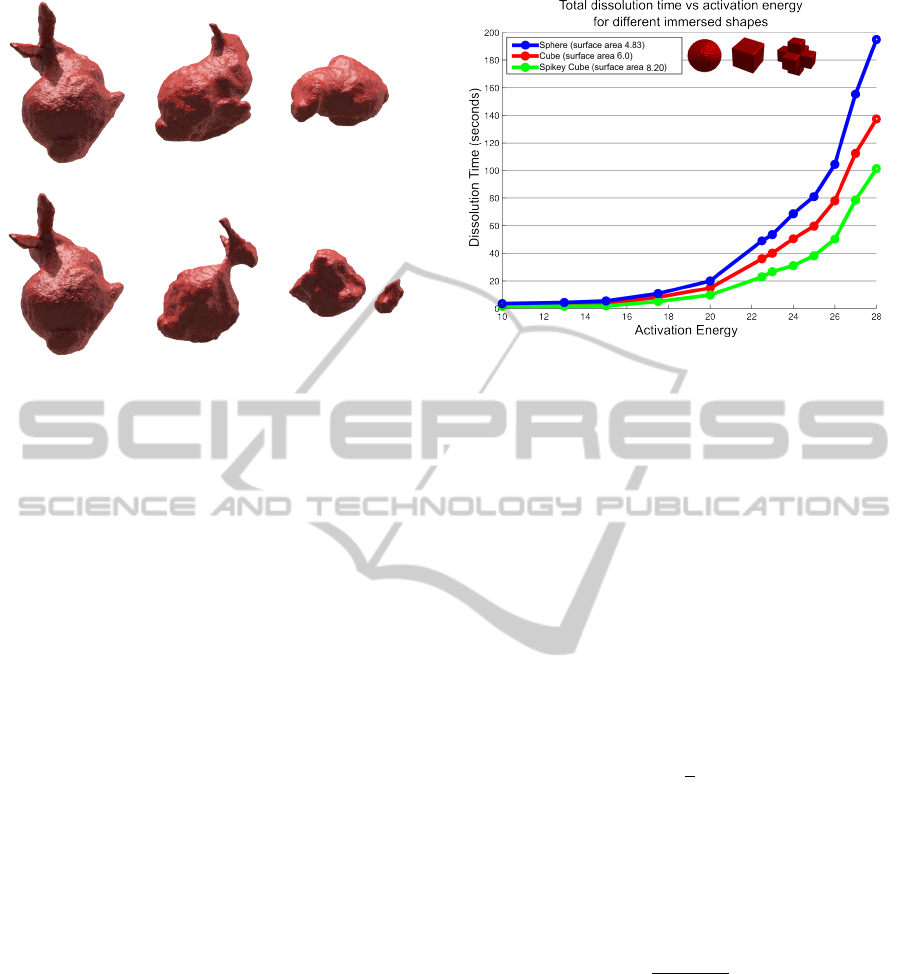
Figure 1: 2D bunny dissolving in ﬂuid. Using our method

(in (a), (b) and (c)) the sampling density does not affect

the dissolution process, even when the sampling is non-

homogeneous. In (d) we demonstrate the result when using

previous methods (Wojtan et al., 2007; Shin et al., 2010).

All the images are taken from the same frame with the same

initial conditions. The solute particles with high energy are

coloured in red.

= v

· ρ

∑

W (x

− x

, h), (2)

where v

and ρ

are respectively the volume and the

representative density of each solid particle. V is

the volume of the entire object and m

is the mass

of each particle: both of which are constant once

the object is initialised. N is the number of par-

ticles used to sample the object. It is easy to tell

that ρ

∑

W (x

−x

, h) originates from the basic

SPH density calculation in Equation 1. j is the object

particle within the solute neighbourhood h. The vol-

ume mass m

must be updated in each frame due to

the changing shape of the object during dissolution.

Figure 1 demonstrates sampling independence

by using different sampling resolutions, as well as

non–homogeneous sampling resolutions, and com-

pare these against previous dissolution methods (Wo-

jtan et al., 2007; Shin et al., 2010). This property is

further discussed in Section 4.2.

3.2.2 Particle Excitation

Particle excitation is measured by local particle en-

ergy. Since collision itself is a kinetic process, we de-

rive our particle excitation equation from the kinetic

energy

, where v is the relative velocity. This is

incorporated into Equation 1 to derive an expression

for particle excitation:

∑

[

+ v

+ ε)]

W (x

− x

, h), (3)

where m

is the volume mass from Equation 2; f

is the solvent particle within the neighbourhood of

solid particle s; m

and ρ

are the mass and density

of ﬂuid particle; v

is the relative linear velocity of

solid and ﬂuid particles; and W (x

− x

, h) is poly6

kernel (M

uller et al., 2003), which smooths out the

energy according to distance; other kernel may apply,

such as cubic spline (Ihmsen et al., 2014).

According to the collision theory, the detachment

of particles only occurs when particles collide with

right angle and enough strength. In SPH, however,

particles cannot collide as they will be repelled by the

pressure between particles. Instead, we consider two

particles to collide once one particle has entered the

neighbourhood of the other. Particles outside of the

neighbourhood are not computed. The size of the ve-

locity is affected by the angle of the collision, calcu-

lated by:

= max((v

− v

) · (x

− x

), 0), (4)

where v

s, f

represent the velocity of solid and ﬂuid

particles respectively. The direction of v

is x

− x

This is illustrated in Figure 2, where only f

and f

contribute to the collision.

Figure 2: The collision domain. s represents a solid parti-

cle and f

1,2,3,4

are ﬂuid particles. The blue arrows indicate

the actual relative velocity, while yellow ones indicate the

calculated linear relation velocity v

represents the angular velocity which con-

tributes to the local particle energy. v

is calculated

by w ×r, where w is the angular velocity and r is the

vector from the particle position to the centre of the

object. This is only needed when there is obvious rel-

ative rotational motion between the object and ﬂuid.

Figure 3 shows the different dissolution behaviours of

the spinning bunny with and without angular velocity.

A small ε is also added to represent the random

thermal motion among molecules (ε = 0.00001 in

our model), which gives the possibility of dissolution

when there is no macroscopic relative motion between

the ﬂuid and solid.

GRAPP2015-InternationalConferenceonComputerGraphicsTheoryandApplications

288

(a) Dissolving without v

(b) Dissolving with v

Figure 3: A spinning bunny dissolves in water. Note that

(b) demonstrates separation behaviour (discussed in Sec-

tion 4.3). The ﬂuid is not rendered in these examples.

accumulates by time: when it is larger than a

user speciﬁed activation energy, the particle dissolves

into the solution. As described by Equation 2, parti-

cles tend to have larger volume mass where the sam-

pling is more compact. This corrects the single par-

ticle energy by making the particle more active (i.e.

larger energy) in Equation 3, making it dissolve faster.

3.3 Activation Energy

The activation energy provides a physically correct

mechanism by which the dissolution rate of individ-

ual particle can be controlled. However, this offers no

control over the time taken for the object to be com-

pletely or partially dissolved: a property that is par-

ticularly important to animators seeking to control the

simulation without having to resort to trial and error.

In this section we provide the bridge to connect the

global dissolution time with the local particle excita-

tion. Dissolution depends on the nature of the solvent

and solute, the temperature of both, the inter–facial

surface area between them, and the presence of mix-

ing (McNaught and Wilkinson, 1997). In our method

the presence of mixing is implicitly solved by the par-

ticle excitation. For simplicity, we assume tempera-

ture to be a constant parameter θ (although this could

be varied within more complex simulations).

We determine the relationship between the total

dissolution time T , activation energy E

and the inter–

facial surface area S based on our simulation experi-

ments. In Figure 4, we show the results of dissolv-

ing objects with different inter–facial surface areas

and different activation energies. The three objects

(sphere, cube, spiky cube) have the same volume. The

Figure 4: The relationship between the total dissolution

time and activation energy for different immersed shapes.

Shapes with more surface area in contact with the ﬂuid nat-

urally dissolve faster. The observed dissolution rates leads

us to use the exponential function to model the total disso-

lution time as a function of activation energy.

surface area is respectively 4.83, 6.0, and 8.20.

Each curve describes the dissolution times of cer-

tain object with different activation energies. The

shape of the curve is best approximated with the gen-

eral exponential function (α = 0.25 in our examples):

T ∝ exp(αE

), (5)

By observing the dissolution time of the different

objects with the same activation energy, the relation-

ship between dissolution time T and surface area S

matches:

T ∝

. (6)

This agrees with common sense: a larger surface area

results in shorter dissolution time.

According to Equations 5 and 6, we can con-

clude that the relationship between the total dissolu-

tion time, activation energy and the inter-facial sur-

face area can be described as:

T =

exp(αE

)

θS

, (7)

Using this experimental methodology, artists are

able to better estimate the total dissolution time for

objects based on the surface area and the local acti-

vation energy. An interactive tool could be developed

which uses preceding simulation results of a partic-

ular ﬂuid conﬁguration to calculate the coefﬁcients

for better estimation. Once the coefﬁcients are de-

termined, the inverse of this function can be used to

determine the activation energy for an artist speciﬁed

target dissolution time.

AParticle-basedDissolutionModelusingChemicalCollisionEnergy

289

3.4 Object Update

The positions of solutes are updated as rigid bod-

ies. Each disconnected component will be treated as

a rigid body, more detail discussed in Section 4.3.

No relative motion is expected among the particles

in one rigid body. The forces acted on the object are

the forces from the ﬂuid, the gravity, and the support

force when the objects hit the boundary. The forces

from ﬂuid, such as pressure and viscosity forces,

equal to the opposite of the corresponding forces from

the object to ﬂuid. The rules updating the solid obey

the same with standard rigid body dynamics (Feath-

erstone, 2007).

4 IMPLEMENTATION AND

RESULTS

We ran our simulations on an Intel Xeon W3680 (8M

Cache, 3.33GHz) with 8GB RAM. The SPH ﬂuid

simulation implemented in CUDA and executed us-

ing a GeForce 460Ti with 1GB onboard RAM. Real–

time results are rendered in OpenGL, and simulation

results were exported and rendered externally using

Houdini. The computational cost of our algorithm is

depending on the number of both solute and solvent

particles, the complexity of interaction between solute

and solvent and the update of solute positions. The

real–time performance of our technique is presented

in Table 1. In a same example, the performance can

be largely improved with less solute particles. There-

fore, our sampling independent dissolution model al-

lows animators to preview the dissolution behaviour

with a lower computational cost. Our method is very

efﬁcient and advantageous for pre-visualization.

Table 1: The performance in average frames per second

(FPS) of our method in different examples. Solute and Sol-

vent represent the number of particles in each.

Example Solute Solvent FPS

Spinning bunny 28553 65535 27

Antacid pills 12745 80000 50

Spheres (low) 8538 100000 148

Spheres (high) 22274 100000 48

River Bed 15000 385948 19

Layered Terrain 169650 262140 20

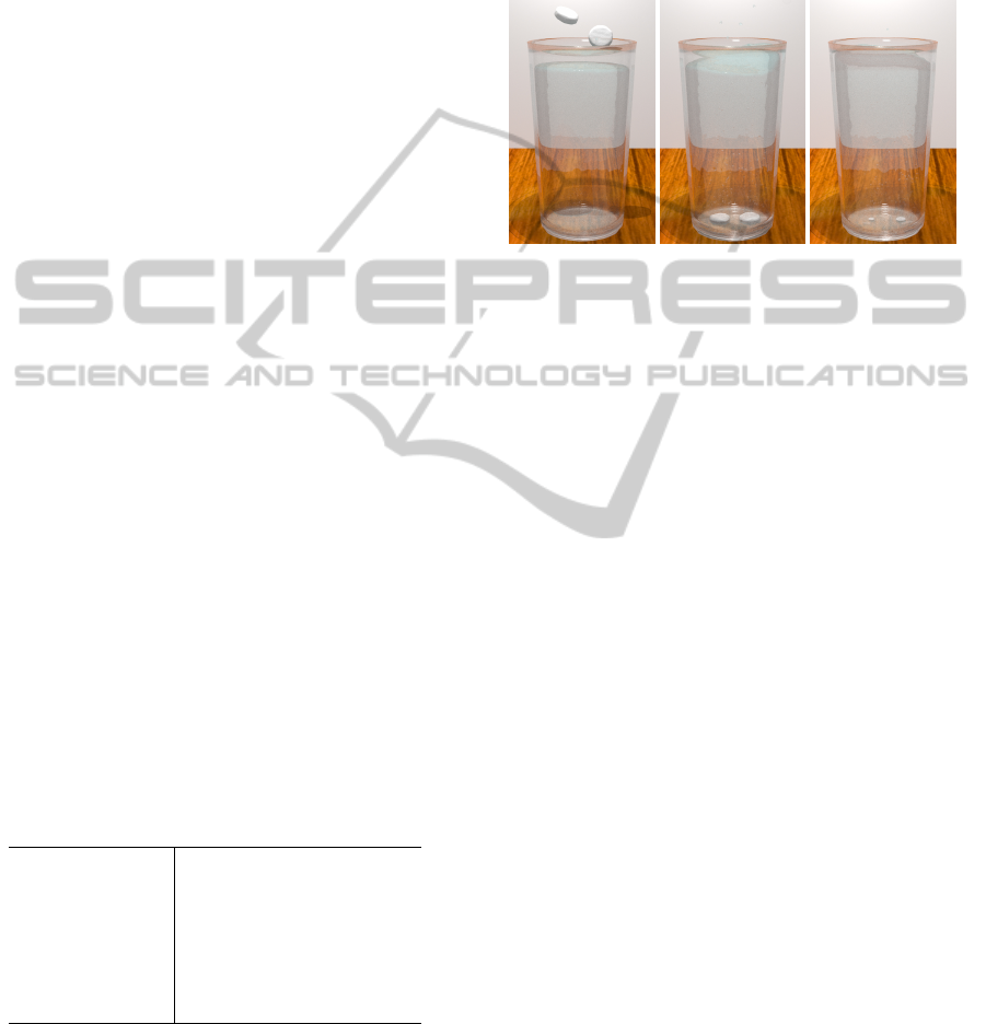
4.1 Antacid Pills to Water

Antacid pills are a classic demonstration of dissolu-

tion behaviour for simulation. In Figure 5 we demon-

strate our effect on two Antacid pills dropped into

a glass of water. Bubbles caused by the release of

trapped air and chemical processes are recognisable

clues that dissolution is taking place. We add bubbles

at the dissolution site to increase the authenticity of

the simulation. The bubble motion is modelled using

basic Brownian motion similar in (Kim et al., 2010).

Figure 5: Two antacid pills dissolving in water.

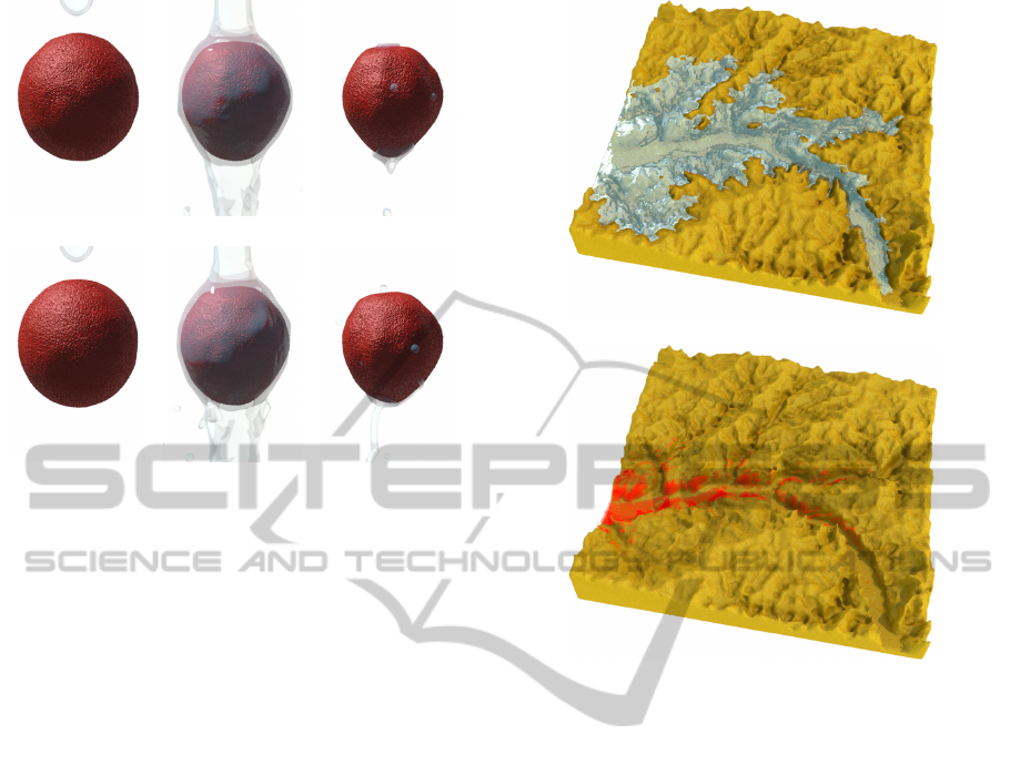
4.2 Sampling Independent Dissolution

In Figure 6 we pour liquid over a sphere, demonstrat-

ing the effect of pouring ﬂuid at a targeted area. We

also evaluate this example using two different sam-

pling resolutions in order to demonstrating that the

dissolution results are equivalent. We calculated the

percentage of the volume difference at each frame of

both spheres: with our method, this reaches a max-

imum of 3.4% of the sphere volume, while with the

method of (Wojtan et al., 2007; Shin et al., 2010)

the low sampled sphere dissolves completely before

the high sampled sphere halves in size. The adhesion

method of (Akinci et al., 2013) is used to ensure the

ﬂuid realistically adheres to the sides of the sphere.

4.3 Separation

During dissolution, parts of object may break off and

form separate shapes. In order to track changes to the

topology of the shape, we use a region growing algo-

rithm to detect the object separation during dissolu-

tion, a method commonly used in image segmentation

(Hojjatoleslami and Kittler, 1995). We apply the tech-

nique to identify connected regions from amongst the

volumetric particles. Particles that are close enough

are grouped into clusters, each representing a separate

rigid body.

The main challenge in implementing this algo-

rithm is testing the proximity of particles, but as we

already have neighbourhood information as part of

the ﬂuid simulation, this becomes trivial. We update

the neighbourhood information before evaluating the

region growing algorithm. The region grows from

a random seed particle p by adding it to cluster C.

GRAPP2015-InternationalConferenceonComputerGraphicsTheoryandApplications

290

(a) Sphere sampled with 8538 particles

(b) Sphere sampled with 22274 particles

Figure 6: Fluid is poured over spheres with different sam-

pling resolutions, with almost identical results, except that

the sphere dissolves more smoothly with higher resolution.

Neighbours of p are added to C. Then all new parti-

cles in C become the new seeds for the next iteration.

Note that only neighbours that are not in C are added.

The algorithm proceeds until there are no more valid

particles that can be added to C — each resulting clus-

ter is a separate body. Implementing this algorithm in

parallel is an interesting area of future research. In

Figure 3(b) the bunny separates into pieces as a result

of the dissolution.

4.4 Erosion

We use our dissolution method to simulate complex

natural erosion phenomena. While we do not use the

actual physical properties of different terrain types,

these examples demonstrate the viability of using our

model for practical simulations. Figure 7 shows the

hydraulic erosion acting on the ﬂoor of a river bed.

As the ﬂuid runs over the terrain, certain soil particles

become dissolved in the water. Note that more com-

plex properties of erosion, such as ﬂuid carrying and

relocating sediment, are ignored in our simulation.

One advantage of our energy based model is that

we can simulate different terrain types by simply

modifying the activation energy of individual layers

of particles. This allows us to simulate erosion of

rocks consisting of different layers each with different

material properties, giving rise to natural formations

similar to those which can be found in mountainous

or coastal regions.

This is demonstrated in Figure 8, where a three

(a) Fluid simulation

(b) Resulting erosion

Figure 7: Hydraulic erosion with dissolution model. In (a)

we show the dissolution process, while in (b) the removed

soil particles are shown in red.

layered terrain is immersed in turbulent ﬂuid to simu-

late coastal erosion. Different activation energies are

assigned to particles in each layer, with the lowest ac-

tivation energy assigned to the middle layer — lead-

ing to a natural arch formation.

5 CONCLUSION

In this paper we introduce a novel energy-based dis-

solution model based on the collision theory. We

demonstrate by way of examples that this method

achieves physically and chemically plausible dissolu-

tion and erosion behaviours. The key to this model

is a new expression for particle excitation based on

kinetic energy. By using the volume mass instead of

mass to update local particle energy, we are able to

ensure the same dissolution results independent of the

sampling density.

We also identify the relationship between global

dissolution time and the local particle activation en-

ergy, allowing animators to easily adjust the global

properties of the dissolution simulation by modify-

AParticle-basedDissolutionModelusingChemicalCollisionEnergy

291

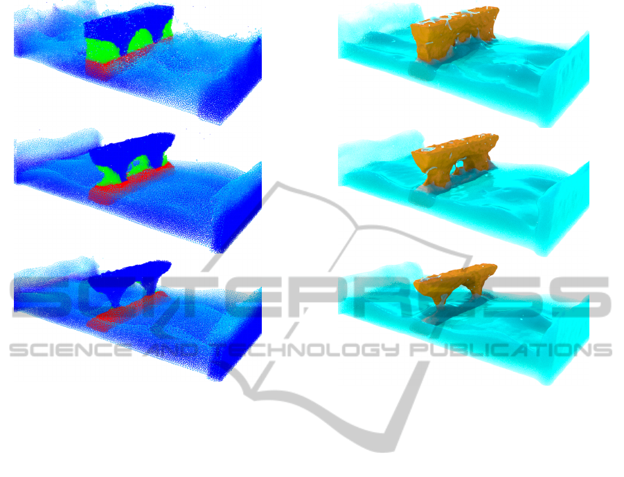
Figure 8: A simulation of layered terrain erosion using our

dissolution model. The solute consists of three different ma-

terial layers, each with a different activation energy. Forces

are added to the ﬂuid to keep the ﬂuid active. This simula-

tion consists of about 430k combined particles and runs as

20 frames per second on a commodity graphics card. Please

refer to Figure 9 for the rendered results.

ing a single parameter. In addition, our method is

straightforward to implement in an existing particle–

based ﬂuid framework, and naturally lends itself to a

parallel implementation.

There are several exciting avenues for research

arising from our energy–based model. The indepen-

dence on sampling resolution implies that adaptively

reﬁning solute representations or multi–grid methods

could be applied to improve the dissolution compu-

tation performance, the incorporation of temperature

into our model will allow for more accurate simula-

tion of melting effects, and the uniﬁed particle nature

of our dissolution model and other recently published

work hints at a uniﬁed representation for interacting

media, allowing gases, solvents and solutes to be sim-

ulated within a single framework.

ACKNOWLEDGEMENTS

We would like to thank Phil Spicer for ﬂuid rendering,

Mathieu Sanchez for providing Signed Distance Field

library, Shujie Deng and Wei Wang for video editing.

Figure 9: Rendered results of layered terrain erosion using

our dissolution model.

REFERENCES

Akinci, N., Akinci, G., and Teschner, M. (2013). Versa-

tile surface tension and adhesion for sph ﬂuids. ACM

Trans. Graph., 32(6):182:1–182:8.

Akinci, N., Ihmsen, M., Akinci, G., Solenthaler, B., and

Teschner, M. (2012). Versatile rigid-ﬂuid coupling for

incompressible sph. ACM Trans. Graph., 31(4):62:1–

62:8.

Amada, T. (2006). Real-time particle-based ﬂuid simulation

with rigid body interaction. In Dickheiser, M., editor,

Game Programming Gems 6, pages 189–205. Charles

River Media.

Arash, O. E., Gnevaux, O., Habibi, A., and michel Dischler,

J. (2003). Simulating ﬂuid-solid interaction. In in

Graphics Interface, pages 31–38.

Batty, C., Bertails, F., and Bridson, R. (2007). A fast vari-

ational framework for accurate solid-ﬂuid coupling.

ACM Trans. Graph., 26(3).

Becker, M., Tessendorf, H., and Teschner, M. (2009). Di-

rect forcing for lagrangian rigid-ﬂuid coupling. IEEE

Transactions on Visualization and Computer Graph-

ics, 15(3):493–503.

Bene

s, B., T

ınsk

y, V., Horny

s, J., and Bhatia, S. (2006).

Hydraulic erosion. Computer Animation and Virtual

Worlds, 17(2):99 – 108.

Busaryev, O., Dey, T. K., Wang, H., and Ren, Z. (2012).

Animating bubble interactions in a liquid foam. ACM

Trans. Graph., 31(4):63:1–63:8.

GRAPP2015-InternationalConferenceonComputerGraphicsTheoryandApplications

292

Carlson, M., Mucha, P. J., and Turk, G. (2004). Rigid

ﬂuid: Animating the interplay between rigid bodies

and ﬂuid. In ACM Trans. Graph, pages 377–384.

Clark, J. (2004). The Essential Dictionary of Science. New

York: Barnes & Noble Book.

Cleary, P. W., Pyo, S. H., Prakash, M., and Koo, B. K.

(2007). Bubbling and frothing liquids. ACM Trans.

Graph., 26(3).

Featherstone, R. (2007). Rigid Body Dynamics Algorithms.

Springer-Verlag New York, Inc., Secaucus, NJ, USA.

Foster, N. and Metaxas, D. (1996). Realistic animation of

liquids. Graph. Models Image Process., 58(5):471–

483.

Gingold, R. A. and Monaghan, J. J. (1977). Smoothed par-

ticle hydrodynamics-theory and application to non-

spherical stars. Monthly Notices of the Royal Astro-

nomical Society, 181:375–389.

Harada, T., Tanaka, M., Koshizuka, S., and Kawaguchi, Y.

(2007). Real-time coupling of ﬂuids and rigid bodies.

APCOM in conjunction with EPMESC XI, (3-6).

Hoetzlein, R. C. (2010-2014). Fast ﬁxed-radius nearest

neighbors: Interactive million-particle ﬂuids.

Hojjatoleslami, S. and Kittler, J. (1995). Region growing:

A new approach. IEEE Transactions on Image Pro-

cessing, 7:1079–1084.

Ihmsen, M., Akinci, N., Akinci, G., and Teschner, M.

(2012). Uniﬁed spray, foam and air bubbles for

particle-based ﬂuids. Vis. Comput., 28(6-8):669–677.

Ihmsen, M., Orthmann, J., Solenthaler, B., Kolb, A., and

Teschner, M. (2014). SPH Fluids in Computer Graph-

ics. pages 21–42.

Kim, D., young Song, O., and Ko, H.-S. (2010). A practical

simulation of dispersed bubble ﬂow. In ACM SIG-

GRAPH 2010 papers, SIGGRAPH ’10, pages 70:1–

70:5.

Kri

stof, P., Bene

s, B.,

Kriv

anek, J., and

Stava, O. (2009).

Hydraulic erosion using smoothed particle hydrody-

namics. Computer Graphics Forum, pages 219–228.

Lucy, L. B. (1977). A numerical approach to the testing of

the ﬁssion hypothesis. Astron. J., 82:1013–1024.

McNaught, A. D. and Wilkinson, A. (1997). Collision the-

ory. Oxford: Blackwell Scientiﬁc Publications.

uller, M., Charypar, D., and Gross, M. (2003).

Particle-based ﬂuid simulation for interactive appli-

cations. In Proceedings of the 2003 ACM SIG-

GRAPH/Eurographics symposium on Computer ani-

mation, SCA ’03, pages 154–159.

Robinson-Mosher, A., Shinar, T., Gretarsson, J., Su, J., and

Fedkiw, R. (2008). Two-way coupling of ﬂuids to

rigid and deformable solids and shells. ACM Trans.

Graph., 27(3):46:1–46:9.

Schechter, H. and Bridson, R. (2012). Ghost sph for ani-

mating water. ACM Trans. Graph., 31(4):61:1–61:8.

Shin, S.-H., Kam, H. R., and Kim, C.-H. (2010). Hybrid

simulation of miscible mixing with viscous ﬁngering.

Comput. Graph. Forum, pages 675–683.

Solenthaler, B. and Pajarola, R. (2009). Predictive-

corrective incompressible sph. ACM Trans. Graph.,

28(3):40:1–40:6.

Solenthaler, B., Schl

aﬂi, J., and Pajarola, R. (2007). A uni-

ﬁed particle model for ﬂuid–solid interactions: Re-

search articles. Comput. Animat. Virtual Worlds,

18(1):69–82.

Stomakhin, A., Schroeder, C., Jiang, C., Chai, L., Teran,

J., and Selle, A. (2014). Augmented mpm for phase-

change and varied materials. ACM Trans. Graph.,

33(4):138:1–138:11.

Trautz, M. (1916). Das gesetz der reaktionsgeschwindigkeit

und der gleichgewichte in gasen. besttigung der

additivitt von cv-3/2r. neue bestimmung der in-

tegrationskonstanten und der molekldurchmesser.

Zeitschrift fr anorganische und allgemeine Chemie,

96(1):1–28.

Wojtan, C., Carlson, M., Mucha, P. J., and Turk, G.

(2007). Animating corrosion and erosion. In Proceed-

ings of the Third Eurographics conference on Natu-

ral Phenomena, NPH’07, pages 15–22, Aire-la-Ville,

Switzerland, Switzerland. Eurographics Association.

AParticle-basedDissolutionModelusingChemicalCollisionEnergy

293