Implicit Shape Models for 3D Shape Classiﬁcation with a Continuous

Voting Space

Viktor Seib, Norman Link and Dietrich Paulus

Active Vision Group (AGAS), University of Koblenz-Landau, Universit

atsstr. 1, 56070 Koblenz, Germany

Keywords:

Implicit Shape Models, 3D Shape Classiﬁcation, Object Recognition, Hough-Transform.

Abstract:

Recently, different adaptations of Implicit Shape Models (ISM) for 3D shape classiﬁcation have been pre-

sented. In this paper we propose a new method with a continuous voting space and keypoint extraction by

uniform sampling. We evaluate different sets of typical parameters involved in the ISM algorithm and com-

pare the proposed algorithm on a large public dataset with state of the art approaches.

1 INTRODUCTION

With the advent of low-cost consumer RGBD-

cameras 3D data of every day’s objects is available

for and can be generated by anyone. However, the

task of recognizing 3D objects is still an open area

of research. Of particular interest is the ability of

3D recognition algorithms to generalize from train-

ing data to enable classiﬁcation of unseen instances of

learned shape classes. For instance, objects belonging

to the class “chair” might exhibit great shape varia-

tions while the general characteristics (sitting plane

and backrest) are present throughout a majority of

class instances. When designing algorithms for 3D

object recognition a balance between implicit shape

description for high intra-class variations and explicit

shape representation to distinguish different classes

needs to be found.

Recently, extensions of the Implicit Shape Model

(ISM) approach to 3D data have become popular. As

the name suggests, an object is not described by a di-

rect representation of its shape. Rather, an implicit

representation is built which enables the algorithm to

cope with shape variations and noise. The original

ISM approach for object detection in 2D by Leibe et

al. (Leibe and Schiele, 2003; Leibe et al., 2004) pro-

posed to represent the local neighborhood by image

patches. Assuming a ﬁxed camera position and no ro-

tations, a window of ﬁxed size is superimposed on the

detected keypoint position to represent the surround-

ing area. An implicit description for an object class is

learned comprising a number of object-speciﬁc fea-

tures and their spatial relations. Object detection is

performed using a probabilistic formulation to model

the recognition process.

The contributions of this work are as follows. In

Section 2 we review recent approaches that extend

the ISM formulation to 3D. Further, in Section 3

and 4 we propose a new extension of ISM to 3D

which differs in the following aspects from recent ap-

proaches. First, we propose to use a continuous 3D

voting space and the Mean-Shift algorithm (Fukunaga

and Hostetler, 1975; Cheng, 1995) for maxima de-

tection as in the original 2D ISM approach. Second,

contrary to other approaches we show that uniformly

sampling keypoints on the input data proves more

beneﬁcial than using a keypoint detector of salient

points. Finally, we include an additional weight into

the voting process that takes into account the similar-

ity of a detected feature and a codeword. Our method

is evaluated regarding the choice of algorithm param-

eters, robustness to noise and compared with other ap-

proaches on publicly available datasets in Section 5.

We conclude the paper and give an outlook to future

work in Section 6.

2 RELATED WORK

Leibe et al. introduced the concept of Implicit Shape

Models (ISM) in (Leibe and Schiele, 2003) and

(Leibe et al., 2004). In their approach keypoints are

extracted using the Harris corner detector (Harris and

Stephens, 1988), while image patches describe the

keypoint neighborhood. These patches are grouped

into visually similar clusters, the so called codewords,

reducing the amount of image patches by 70 %. The

Seib V., Link N. and Paulus D..

Implicit Shape Models for 3D Shape Classiﬁcation with a Continuous Voting Space.

DOI: 10.5220/0005290700330043

In Proceedings of the 10th International Conference on Computer Vision Theory and Applications (VISAPP-2015), pages 33-43

ISBN: 978-989-758-090-1

 2015 SCITEPRESS (Science and Technology Publications, Lda.)

set of codewords is referred to as the codebook. The

possible locations on the object are obtained by com-

puting vectors from the object center to features that

are similar to at least one of the codewords. These

activation vectors and the codebook form the ISM for

the given object class. the extracted image patches of

a test image are matched with the codebook. While

the activation vectors have initially been generated

from image patch locations in relation to the known

object center, this information is used to derive hy-

potheses for object locations. Hence, each codeword

casts a number of votes for a possible object location

into a voting space. Object locations are acquired by

analyzing the voting space for maxima using Mean-

Shift Mode Estimation (Cheng, 1995).

In analogy to image patches with a ﬁxed window

size in 2D, a subset of the input data within a spec-

iﬁed radius around the interest point represents the

local neighborhood in 3D. Typically, the SHOT in-

terest point descriptor (Tombari et al., 2010) is used.

However, other descriptors like the extension of the

original SURF descriptor (Bay et al., 2006) to 3D

also prove beneﬁcial (Knopp et al., 2010b). While

the original approach did not consider rotation invari-

ance, this feature is highly desirable for 3D since ob-

jects might be encountered at different poses or views.

An early extension of ISM to 3D is described by

Knopp et al. (Knopp et al., 2010b). The input fea-

ture vectors from 3D-SURF are clustered using the k-

means algorithm. As a heuristic, the number of clus-

ters is set to 10 % of the number of input features.

Codewords are created from centers of the resulting

clusters. Scale invariance is achieved by taking into

account a relative scale value derived from the fea-

ture scale and the object scale. Before casting votes

into the voting space votes are weighted to account

for feature-speciﬁc variations. Detecting the class of

a test object requires analyzing the 5D voting space

(3D object position, scale and class) for maxima.

Knopp et al. do not address rotation in (Knopp

et al., 2010b), but discuss approaches to solving rota-

tion invariant object recognition for Hough-transform

based methods in general in (Knopp et al., 2010a).

The problem is divided into three categories, depend-

ing on the additional information available for the in-

put data. In case a local reference frame is avail-

able for each feature point voting transfers an object-

speciﬁc vote from the global into a local reference

frame during training and vice versa during detection.

If only the normal at each feature is available vote po-

sitions are conﬁned to a circle around the feature with

the normal direction (circle voting). If neither nor-

mals nor local reference frames are available, sphere

voting conﬁnes the vote position to a position on a

sphere. Regions with high density in the voting space

are then created by voting circle and sphere intersec-

tions, respectively.

While circle and sphere voting is a suitable

method our own experiments showed several disad-

vantages. Circles and spheres need to be subsampled

in order to contribute to the voting space. To guaran-

tee equal point distributions independently from fea-

ture locations the sampling density needs to increase

with the radius. Thus, the point concentration in the

voting space will increase with the object size. How-

ever, precise maxima are difﬁcult to extract in an over-

sampled voting space and circles and spheres close

to each other promote the creation of irrelevant side

maxima and strengthen false positives. Due to these

disadvantages we decided to compute local reference

frames for each detected feature in our approach.

Contrary to Knopp et al. (Knopp et al., 2010b),

Salti et al. claim that scale invariance does not need to

be taken care of, since 3D sensors provide metric data

(Salti et al., 2010). In their approach Salti et al. inves-

tigate which combinations of clustering and codebook

creation methods are best for 3D object recognition

with ISM. Following their results, a global codebook

with k-means clustering leads to best results. As de-

scriptor, Salti et al. suggest SHOT (Tombari et al.,

2010) because of its repeatability and a provided lo-

cal reference frame.

A more recent approach presented by Wittrowski

et al. (Wittrowski et al., 2013) uses ray voting in

Hough-space. Like in other ISM adaptations to 3D

a discrete voting space is used. However, in this ap-

proach bins are represented by spheres which form di-

rectional histograms towards the object’s center. This

voting scheme proves very efﬁcient with an increas-

ing number of training data. While other methods

store single voting vectors in codewords, here only

histogram values needs to be incremented.

3 CREATING THE IMPLICIT 3D

SHAPE MODEL

The ISM framework consists of two parts: the train-

ing and the classiﬁcation stage. In both cases some

preprocessing on the input data is necessary.

First, consistently oriented normals on the input

data have to be determined. If the input data con-

sists of a single view of the scene, normals can be ori-

ented toward the viewpoint position. However, many

datasets consist of full 3D models of objects acquired

from several different viewpoints. To compute consis-

tently oriented normals on such a set of unorganized

points we apply the method proposed by Hoppe et al.

VISAPP2015-InternationalConferenceonComputerVisionTheoryandApplications

(Hoppe et al., 1992).

After normal computation, representative key-

points are detected on the data and a local refer-

ence frame is computed for each keypoint. Then, a

descriptor representing properties of the local key-

point neighborhood is computed for each keypoint

in the previously determined local reference frame.

We evaluated our approach with three different key-

point extraction methods and three different descrip-

tors. More details are presented in Section 5.

In the context of Implicit 3D Shape Models, we

deﬁne a feature f as a triple, composed of a keypoint

position p

, a local descriptor l

with dimensionality

n and a representation of the local reference frame,

given by a rotation matrix R

f = hp

, R

, l

i (1)



, p



∈R



x y z



∈R

3×3



, l

, . . . , l



∈R

For a given class C, a feature detected on an in-

stance of C is denoted by

= hp

, R

, l

i. (2)

Finally, the set F represents all detected features

on a scene

F = {f

C,i

} ∀C. (3)

3.1 Clustering and Codebook

Generation

After computing features on the training data, a code-

book is created by clustering features according to

their corresponding descriptors into codewords. The

process of codebook creation is illustrated in Figure

1. While the original ISM used image patches to de-

scribe the local properties of an object, in our case

codewords represent the local geometrical structure.

Thus, features are clustered based on the geometrical

similarity of their corresponding object regions. The

resulting cluster centers represent prototypical local

shapes independently from their positions on the ob-

ject.

Salti et al. (Salti et al., 2010) distinguish two

types of codebooks. A local codebook treats each

object class individually: the features of the training

models for each object class are clustered to create

a class-speciﬁc codebook. During detection, a sepa-

rate codebook is used for each of the object classes.

It is likely that a codebook contains codewords that

are similar to codewords of a different codebook for a

different class. In contrast, a global codebook is com-

puted over all detected features in all classes. Features

Figure 1: Training pipeline: Features are extracted on the

initial training model and clustered by their similarity to

create codewords in a codebook. The features are then

matched with the codebook according to an activation strat-

egy to create a spatial distribution of codeword locations.

Codebook and activation distribution represent the trained

Implicit Shape Model.

from all classes contribute to the representation for a

speciﬁc object class. Thus, using a global codebook

approach allows for a wider generalization. During

detection, the codebook is shared among all object

classes. Motivated by the results provided by Salti

et al. (Salti et al., 2010), the approach presented here

uses a global codebook.

Clustering is performed with the k-means cluster-

ing algorithm. One of the main drawbacks of k-means

clustering is the choice of k, which is not trivial. Sev-

eral approaches exist to determine k automatically.

Simple solutions estimate k from the size of the data

set. Several rules of thumb such as k = m kX k as

mentioned by Knopp et al. (Knopp et al., 2010b) ex-

ist, assuming a certain percentage of the data size for

k and referring to m as the cluster factor. However, the

precise choice of k is not critical in this context, since

the exact number of partitions can not be precisely de-

termined for the high-dimensional descriptor space.

Slight variations in the clusters are not crucial to the

algorithm, as long as the cluster assignment works as

expected and the within-cluster error function is effec-

tively minimized. Using the above described heuristic

is therefore sufﬁcient for the current approach.

After clustering, the created codebook C contains

a list of codebook entries (codewords) c

∈ R

, rep-

resented as cluster centers from feature descriptors

∈ R

C = {c

, c

, . . . , c

| c

∈ R

}. (4)

3.2 Codeword Activation

So far, the codebook contains a list of codewords

which are prototypical for a speciﬁc geometrical

property of the training model. However, the code-

book does not contain any spatial information, yet. In

accordance with the Implicit Shape Model formula-

tion in (Leibe and Schiele, 2003), the activation step

builds a spatial distribution specifying where each

ImplicitShapeModelsfor3DShapeClassificationwithaContinuousVotingSpace

Figure 2: Activation procedure during training. Detected

features activate a codeword (red) and their relative vectors

to the object center are computed. Based on the local ref-

erence frame associated with each of the features, the vec-

tors are rotated into a uniﬁed coordinate system. The list of

rotated activation vectors then builds the activation distribu-

tion for the current codeword.

feature belonging to a codeword is located on a train-

ing model. By iterating again over all detected fea-

tures, the activation step matches the features with the

generated codewords contained in the codebook ac-

cording to an activation strategy. This strategy spec-

iﬁes whether or not a feature activates a codeword

and is based on a distance measure between feature

and codeword. Since codewords have been created

as cluster centers from a clustering method applied

to feature descriptors, both are given in the same de-

scriptor space. Thus, the activation strategy can work

with the same distance measure as was used by the

clustering method during codebook creation. Given

a feature f

∈ F and the codebook C , the activation

step returns those codewords that match the feature

according to the chosen strategy. The distance be-

tween feature descriptor and codeword is determined

by the distance function d(l

, c) = kl

−ck

The simplest method of activation would activate

only the best matching codeword for the current fea-

ture. However, during codebook creation a multitude

of features has been grouped together to form one

codeword. While all features that have been grouped

together in a codeword have a low distance toward

each other, there is still variation involved in the cor-

rect cluster assignment. It is thus suitable to enable

the activation of more than one codeword, e.g. by ac-

tivating all codewords with a distance to the cluster

below a threshold. In the presented approach we use

the k-NN strategy, where the k best matching code-

words are activated.

For each activated codeword the activation then

creates a spatial distribution specifying where each

codeword is located on the object. First, the keypoint

positions have to be transferred from global coordi-

nates into an object centered coordinate frame. In

order to do this a minimum volume bounding box

(MVBB) of the object is calculated. According to

(Har-Peled, 2001), computing the MVBB is reduced

to ﬁrst approximating the diameter of the point set,

i.e. ﬁnding the maximum distance between a pair of

points p

and p

. The estimated MVBB is then given

by the direction between the diameter points and the

minimum box enclosing the point set, as described

in (Barequet and Har-Peled, 2001), thus yielding an

oriented box B with size s

, center position p

and

identity rotation R

B = hs

, p

, R

i (5)

= p

−p

∈R

= p

∈R

= I

3×3

∈R

3×3

The bounding box is stored with the training data

and used at detection for further analysis. The con-

tained rotation matrix can be used at detection to de-

termine the relative rotation of an object between two

scene views. The object’s reference position is now

given by p

as the center position of the minimum

volume bounding box. The relative feature position is

then given in relation to the object position p

rel

= p

−p

(6)

and represents the vector pointing from the location of

the feature on the object to the object center position.

To allow for rotation invariance, each feature was as-

sociated with a unique and repeatable reference frame

given by a rotation matrix R

. Transforming the vec-

tor v

rel

from the global into the local reference frame

can then be achieved by

= R

·v

rel

. (7)

We obtain v

, the translation vector from the fea-

ture location to the object center in relation to the

feature-speciﬁc local reference frame, as described by

(Knopp et al., 2010a). Thus, v

provides a position

and rotation independent representation for the occur-

rence of feature f (Figure 2). The ﬁnal activation dis-

tribution for a codeword c is then given by

= {v

| ∀f

∈ F

} (8)

where F

is a set containing all features that activated

the codeword c. The set V

contains a list of activa-

tion vectors for codeword c pointing from the feature

location on the object to the object’s center.

In combination with the codebook C , the ﬁnal ac-

tivation distribution maps each codeword c ∈ C to its

list of activation vectors V

and builds the ﬁnal data

pool for the detection process with the activation dis-

tribution for all codewords V . Along with the activa-

tion vectors, each entry in the activation distribution

also stores additional information like the class C of

the feature that activated the corresponding codeword

and the computed bounding box B.

VISAPP2015-InternationalConferenceonComputerVisionTheoryandApplications

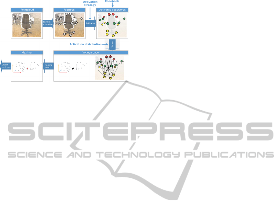
Figure 3: Classiﬁcation pipeline: Features are extracted on

the input point cloud. Detected features are matched with

the codebook and matching codewords cast their activation

vectors into a voting space. When an object is found, acti-

vation vectors build clusters in the voting space, which are

detected by searching for maximum density regions.

4 3D OBJECT CLASSIFICATION

The training process created an implicit object rep-

resentation, consisting of a codebook of local geo-

metrical codewords C and an activation distribution,

reﬂecting the positions where each codeword is ex-

pected to be located on the object. To classify objects,

features are detected on the input point cloud in the

same manner as in the training stage. Matching de-

tected features with the previously trained codebook

yields a list of activated codewords that cast their ac-

tivation vectors into a continuous voting space. When

an object matches one of the representations stored

within the ISM, several activation vectors will cre-

ate clusters at nearby locations. These voting clus-

ters represent hypothetical bounding box centers of

yet unknown object instances. By searching for these

maximum density regions, all object hypotheses are

collected and evaluated using a weighting strategy.

Figure 3 presents an overview of the classiﬁcation

pipeline.

4.1 Codeword Activation

Although technically possible to do otherwise, key-

points are detected here using the same keypoint de-

tection algorithm as was used in training. However,

using the same descriptor is inevitable, since descrip-

tors originating from different methods are formu-

lated in a different descriptor space accounting for

different geometrical properties and thus are not com-

parable by design.

After detecting features, the same activation strat-

egy is employed as was used in training. By match-

ing features with codewords, the activation yields a

number of codewords and their corresponding activa-

tion vectors. Thus, correspondences are established

at locations where the input data is assumed to match

the trained object models. Based on the stored ac-

tivation distribution all activation vectors are subse-

quently collected for each of the activated codewords.

4.2 Weighted Voting

The activation distribution was created to reﬂect all

observed locations on the training object where the

corresponding activated codeword was found. During

voting this process is reversed to back project the ac-

tivation vectors from the activated feature locations to

indicate possible object center locations.

Each activated codeword casts its votes for pos-

sible object locations into a multi-dimensional vot-

ing space. To reduce the dimensionality of the vot-

ing space the object’s rotation is ignored in this step.

Further, a separate voting space for each class reduces

the voting space dimensionality to three, the 3D posi-

tion of the hypotheses. The number of object classes

is known from the training stage.

The voting space for a speciﬁc class is built as a

continuous three-dimensional space, in which every

point is assigned a weight. Each activation vector v ∈

V casts a vote for an object hypothesis into the voting

space at a location x, weighted by ω based on the class

C from the training process. The respective weight

corresponds to the probability that this vote reﬂects

the actual object location. The weight calculation is

explained in the following Section.

After voting, the voting spaces are analyzed for

maxima individually. In each voting space maxima

are selected using the Mean-Shift algorithm described

by Fukunaga and Hostetler (Fukunaga and Hostetler,

1975). Given the ﬁnal object position and class, rota-

tion is estimated as described in Section 4.4.

4.3 Weighting

The probabilistic formulation is implemented using a

weighted voting space. Each vote v being cast gets

therefore an additional weight ω ∈ [0, 1] that models

the probability that this vote supports the correct ob-

ject hypothesis. The maxima represent a region in the

voting space with the highest probability density, i.e.

all votes around the maximum contribute with their

weights to the ﬁnal probability for the object occur-

rence. The ﬁnal vote weight ω for vote v is composed

of three separate individual weights.

Two of these weights, the statistical weight and

the center weight, are adapted from Knopp et al.

(Knopp et al., 2010b). The statistical weight, denoted

ImplicitShapeModelsfor3DShapeClassificationwithaContinuousVotingSpace

, is used to normalize the individual votes. It guar-

antees that the probability is computed independently

from the actual number of votes. The weights are nor-

malized based on the number of activated codewords

and activation vectors. The weight ω

weights a vote

for a class C, created from a codeword c, by

(C)

vot

(c)

vot

(C,c)

f tr

(C)

∑

vot

,c)

f tr

)

. (9)

The ﬁrst and second term normalize the vote weight

by the number of codewords n

current object class C and by the number of votes

vot

third term normalizes on inter-class level. It repre-

sents the probability that the word c votes for the

given class in contrast to the other classes.

The center weight, denoted ω

cen

, is computed for

each vote during training. When creating the activa-

tion distribution the number of activated codewords

per feature depends on the activation strategy. Con-

sequently, not every voting vector assigned to a code-

word points exactly to the true object position. The

weight ω

cen

thus computes the distances from each

entry in the activation distribution v

to the actual ob-

ject center p

cen

= median



exp



−

d(v

, p

)

cen



. (10)

In case a codeword contains a number of votes for a

training model, only those votes that actually fall into

the surrounding of the known object center position

are assigned a high weight. Experiments showed that

cen

= 0.25 is a reasonable value.

As an additional weight, we use the matching

weight, ω

mat

. It represents the matching score be-

tween a feature and the activated codeword. A low

distance represents a higher probability that the fea-

ture matches the current codeword regarding its geo-

metrical properties. Given the feature f with descrip-

tor l

and the corresponding matched codeword c, the

matching weight is given by

mat

= exp



−

dist(l

, c)

2σ

mat



. (11)

Since the distance between feature and codeword is

given in descriptor space, the value of σ

mat

depends

on the chosen descriptor type and indicates how much

a codeword can differ from a feature. The value σ

mat

is determined during training by the sample covari-

ance. Given F

, the features on a training model for a

class C, the sample mean of distances is computed by

µ =

∑

i=1

∑

j=1

dist(l

, c

) (12)

over all features f ∈ F

and activated codewords c

where M = kF

k is the number of found features for

a class C and N are all activated codewords. The ﬁnal

value of σ

mat

is computed as the sample covariance

mat

MN −1

∑

i=1

∑

j=1

(dist(l

, c

) −µ)

. (13)

This value is stored during training and computed in-

dividually for each class. For classiﬁcation the match-

ing weight is evaluated for each vote and σ

mat

is cho-

sen based on the class. The ﬁnal weight assigned to

each vote is a combination of the individual weights:

= ω

·ω

cen

·ω

mat

. (14)

4.4 Rotation Invariance

The activation vector v

rel

of feature f has been rotated

into the local reference frame given by the rotation

matrix R

during training as shown in Eq. (7). During

classiﬁcation the rotation is reversed by the inverse

rotation matrix R

f −1

= R

f T

computed from f on the

scene, resulting in the back rotated activation vector

ˆv

rel

= R

f T

·v

. (15)

The activation vector v

has been created during train-

ing pointing from the feature position to the object

center. The back rotated activation vector for each

feature is used to create an object hypothesis at posi-

tion x relative to the position p

of the detected feature

x = p

+ ˆv

rel

. (16)

Since the activation vector was created in relation to

the center of the bounding box, the object hypothesis

is also the center position of the yet unknown object

and its bounding box (Figure 4). Applying rotation

during training and back rotation during classiﬁcation

the ﬁnal object vote is considered rotation invariant

under the assumption that the computation of the local

reference frame itself is rotation invariant.

4.5 Maxima Search in Voting Space

The approach to detect maximum density regions

within the voting space has been adapted from Hough

and Arbor (Hough and Arbor, 1962) where it was

used to detect straight lines in images. Ballard

(Ballard, 1981) generalized this method to detect

arbitrary shapes. The voting space is a Cartesian

space in which the object’s center is located. It

is subdivided into discrete bins of a certain size.

When an object hypotheses falls into a certain bin

the value of this bin is incremented by the vote’s

VISAPP2015-InternationalConferenceonComputerVisionTheoryandApplications

Figure 4: Activation procedure during detection. Code-

words (red and green) are associated with list of activation

vectors during training. Each vector has been rotated into

the local reference frame of the activating training feature.

Each detected feature in an unknown scene is associated

with its own local reference frame. Features that match the

codebook according to the activation procedure then cast

the corresponding back rotated votes into the voting space,

creating clusters when objects are found.

weight. Maxima in the voting space are detected by

applying non-maximum suppression and choosing

the remaining maximum bins by their accumulator

value. Bins with high accumulator values correspond

to object locations with a high probability, while low

accumulator values can be discarded as irrelevant.

Although easy to implement this discrete voting

space approach has several disadvantages. The

extent of the accumulator bins highly inﬂuences the

precision of the detected object locations. Votes

of different objects might fall into the same bin or

likewise, votes for one object might be scattered

across several bins. Maxima search might then

dismiss the corresponding object if the individual

accumulator values are too small. We therefore use a

continuous voting space without discrete bins.

The voting space created from activation can

be seen as a sparse representation of a probability

density function. While each vote that has been cast

into the voting space represents a probability that

the object is located at the vote position, ﬁnding the

actual object location from the multitude of votes in

the voting space is reduced to ﬁnding those locations

in the probability distribution that have the highest

probability density. In this context, maxima in the

probability density functions are detected using the

Mean-Shift algorithm described by Fukunaga and

Hostetler (Fukunaga and Hostetler, 1975).

Given a point x ∈ R

, the Mean-shift vector

applies the kernel proﬁle g to the point differences

between all neighboring points x

within the kernel

bandwidth h. Since we search for maxima in the

voting space, the data points are the individual votes.

We use a modiﬁed Mean-Shift vector as proposed

by Cheng (Cheng, 1995) to account for weighted

votes. Here, the kernel density gradient estimation is

applied over a weighted point set in which each data

point x is assigned a weight ω ∈ R. The resulting

Mean-Shift vector

Figure 5: Detection process and bounding box extraction.

Left: Computed features and their corresponding local ref-

erence frames. Right: Activated features cast votes into the

voting space. The Mean-Shift Mode Estimation extracted

the predicted object location and the bounding box has been

averaged from the contributing votes.

h,g

(x) =

∑





x−x





∑





x−x





−x (17)

at position x points in the direction of the maximum

density region for the chosen bandwidth. Maxima are

obtained by iteratively following the direction of m

h,g

To create seed points for the Mean-Shift algorithm a

regular grid is superimposed on the data. Each cell

containing at least a minimum number of data points

creates a seed point. Here, the grid size was chosen

√

since the corresponding cell is then perfectly

covered by the kernel.

It is likely that several seed points converge to the

same position. In order to retrieve individual maxima,

a following pruning step performs a non-maximum

suppression and eliminates duplicate maxima. Addi-

tionally, the ﬁnal probability for the detected maxi-

mum at x

max

is given by the kernel density estimation

at the maximum position in the voting space.

4.6 Bounding Box Extraction

During training the bounding box information has

been stored as additional information for each com-

puted vote. Since a vote is generated by matching a

feature to a codeword, the corresponding feature is

associated with a local reference frame.

During classiﬁcation, all detected features on the

unclassiﬁed point cloud that activate a codeword cast

a number of votes into the voting space. When cast-

ing the votes the associated bounding boxes are trans-

ferred back into the global coordinate system using

the corresponding local reference frame for the cur-

rent feature. After maxima detection yields the most

likely object hypotheses all votes that contributed to

the hypothesis and lie around the maximum location

within the kernel bandwidth are collected (Figure 5).

This results in a list of bounding box hypotheses, each

ImplicitShapeModelsfor3DShapeClassificationwithaContinuousVotingSpace

of which has been weighted according to the corre-

sponding vote weight.

Estimation of the bounding box is performed by

creating an average bounding box representation on

the basis of the collected weighted votes, enforcing

the constraint

∑

= 1. While averaging the bound-

ing box size can easily be done, computing an aver-

age weighted rotation is more complex. The rotation

matrix is converted into a quaternion representation.

Averaging quaternions is achieved by computing the

4 ×4 scatter matrix

M =

∑

i=1

(18)

over all quaternions q

and their associated weights

. After computing the eigenvalues and eigenvec-

tors of M, the eigenvector with the highest eigen-

value corresponds to the weighted average quaternion

(Markley et al., 2007).

5 EXPERIMENTS AND RESULTS

In this Section the proposed approach is analyzed

with respect to performance and precision and applied

to several datasets and test cases. Evaluation is per-

formed on two different datasets that are shortly in-

troduced.

Kinect dataset: We created a dataset from Kinect

data in our lab. For each training model, several dis-

tinct scans from different viewpoints have been cap-

tured. The different point clouds for each objects

were aligned manually to create a full 3D training

model. The aligned point clouds were merged and

the resulting point cloud was sampled with a uniform

grid to create a uniform point distribution. Finally,

the point cloud was smoothed with Moving Least

Squares (Alexa et al., 2003) in order to compensate

for noise on the object surface and ﬁltered using a sta-

tistical outlier removal method. Three object classes

were chosen: chairs, computers, tables. Aim@Shape

Watertight dataset (SHape REtrieval Contest 2007,

2014; A Benchmark for 3D Mesh Segmentation,

Princeton University, 2014): This publicly available

dataset contains 20 object classes, each with 20 in-

stances. The ﬁrst 10 objects of each class were used

for training while the remaining 10 were used for

classiﬁcation. Our algorithms uses the point cloud

data type, however this dataset is available as mesh

ﬁles. For evaluation, we converted the meshes to

point clouds and scaled each model to the unit circle.

Table 1: Minimum distance between ground truth and de-

tected object hypothesis (in meters).

PFH FPFH SHOT

Harris3D 0.073 0.192 0.391

ISS 0.072 0.067 0.066

Uniform Sampling 0.075 0.056 0.062

Table 2: Distance between ground truth and most signiﬁcant

object hypothesis (in meters).

PFH FPFH SHOT

Harris3D 1.289 1.585 1.597

ISS 0.882 1.189 1.174

Uniform Sampling 1.116 0.056 0.062

5.1 Selection of Keypoint Detectors and

Descriptors

Before analyzing the performance of the algorithm on

several test cases, the effects of parameter selection

are evaluated. A crucial question is how keypoints

should be selected and which descriptor should be

used. In our experiments we tested the combination

of three different descriptors, PFH (Rusu et al., 2008),

FPFH (Rusu et al., 2009) and SHOT (Tombari et al.,

2010) with three different keypoint selection methods,

Harris3D (Sipiran and Bustos, 2011), Intrinsic Shape

Signatures (ISS) (Zhong, 2009) (in our case used only

as detector) and uniform sampling.

For the given evaluation, the ISM has been trained

with one model only and the detection algorithm has

been applied to a scene containing a single instance

of the trained model. In particular, a chair model

from the Kinect dataset has been trained and detec-

tion was performed on a scene containing the same

chair in front of a wall and a partially visible shelf

and table close to the chair. Detecting the object in

this scene resulted in several hypotheses on the true

object location. Table 1 depicts the minimum distance

of a hypotheses to the ground truth object center de-

pending on different combinations of keypoint detec-

tor and descriptor. We consider an object as correctly

detected if the distance to the ground truth does not

exceed 0.1m.

While the Harris3D detector does not work well

with FPFH and SHOT, all other combinations are ac-

ceptable. However, this analysis does not allow any

conclusions to the signiﬁcance of the object hypothe-

sis. The algorithm detects maxima in the voting space

and computes a probability for each detected object

hypothesis, based on the total weights of all contribut-

ing votes. The detection result is represented by a

list containing each object hypothesis sorted by the

computed probability. Therefore, Table 2 additionally

VISAPP2015-InternationalConferenceonComputerVisionTheoryandApplications

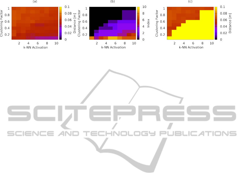
Figure 6: Detection precision plot with one trained object and a scene containing one instance of that object. (a) Minimum

distance to ground truth. (b) Corresponding index in the detection list for hypothesis with minimum distance to the ground

truth. (c) Distance to ground truth of highest weighted hypothesis.

shows the distance to the ground truth of the high-

est weighted and thus most probable object hypothe-

sis. Only the uniform sampling keypoint extraction in

combination with the FPFH or SHOT descriptor leads

to a detected object that is within the acceptable mar-

gin of 0.1 m. Further, these are not only the highest

weighted hypotheses, but also the closest ones to the

ground truth.

The sparse keypoints detected by the Harris3D

and the ISS interest point detector created codewords

with only little votes. Since the process of match-

ing codewords to keypoints suffers from sensor noise,

maxima composed of only few votes are scattered

around in the voting space. In contrast to common

keypoint detectors, uniform sampling takes its advan-

tages from the vast amount of keypoints causing max-

ima in the voting space to be composed from lots of

votes, therefore stabilizing detected maxima. In the

following experiments we use the combination of uni-

form sampling for keypoint extraction and the SHOT

descriptor. SHOT was chosen over FPFH for its run-

time performance.

5.2 Codebook Creation

One interesting aspect is the relationship between

clustering during codebook creation and the activa-

tion strategy. In order to visualize the relationship

between these parameters, training and classiﬁcation

were performed multiple times with different parame-

ter instances. Training was performed using k-means

clustering and the k-NN activation strategy. For clus-

tering, the number of clusters and therefore code-

words was iteratively changed from 100 % to 10 % of

the number of extracted keypoints. At the same time,

the number of activated codewords per feature was

changed from 1 to 10. As before, the result is a list of

object hypotheses sorted by their weight.

Figure 6 (a) shows that for each combination of

k and cluster count, the minimum distance between

the ground truth and the detected object hypotheses

is always within the speciﬁed margin of 0.1 m. The

black area in Figure 6 (b) depicts the cases in which

the object with minimum distance to ground truth is

also the topmost entry in the detection list (highest

weighted object hypothesis). While the data in Figure

6 (a) suggested that the precision improved with in-

creasing k and decreasing cluster count, Figure 6 (b)

suggests that in those cases the object signiﬁcance de-

creases. Figure 6 (c) depicts the ground truth distance

for the highest weighted maxima. The graph shows

that for the best detected hypothesis the distance to

the ground truth is below 0.1 m in all cases.

In each test 1 to 4 chairs were trained while detec-

tion was performed on the same scene as in Section

5.1. Since the results in all these test cases were simi-

lar, we conclude that an increasing number of training

models does not have signiﬁcant effects on the mini-

mum distance to the ground truth.

We further conclude that the best detection preci-

sion is achieved when the activation strategy activates

only a small number of codewords while using a code-

book with only little or no clustering at all. These

results conﬁrm the implications of Salti et al. (Salti

et al., 2010) that the codebook size is not expected

to have any positive inﬂuence on the detection capa-

bilities of the algorithm, but is rather legitimated by

performance considerations. The reason is that with

increasing k each feature activates the k best match-

ing codewords and therefore creates lots of (probably

less signiﬁcant) votes from the corresponding code-

words. Further, with decreasing cluster count more

features are grouped together to create a codeword.

Consequently, even highly different features activate

the same codeword. For the following experiments

we consider only k-NN activation strategies with k

∈ {1, 2, 3} and clustering factors of 1, 0.9 and 0.8.

5.3 Generalization and Inﬂuence of

Noise

We evaluated the ability of our approach to classify

trained objects with different levels of Gaussian noise,

as well as the generalization capability of the ap-

proach. For this task we use scenes containing only

ImplicitShapeModelsfor3DShapeClassificationwithaContinuousVotingSpace

0.6

0.65

0.7

0.75

0.8

0.85

0.9

classification rate

point density (cm)

SHOT radius (cm)

20 25 30

0.25

2.00

1.50

1.00

0.50

20 25 30 20 25 30 20 25 30 20 25 30

test case (A)

test case (B)

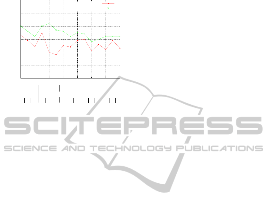
Figure 7: Classiﬁcation results for various point densities

and SHOT radii on the Aim@Shape Watertight dataset. In

test case (A) the same grid size for uniform sampling was

used during training and classiﬁcation. In test case (B) the

grid size during classiﬁcation was equal to half the grid size

from the training step.

the segmented object to be classiﬁed. In the pre-

sented test cases, the training objects from the Kinect

dataset have bee rotated and translated randomly and

Gaussian noise was applied with increasing values

for sigma. The ISM has been trained on all avail-

able training objects. However, two different training

cases have been chosen. In case (A) several objects

were assigned the same class. In particular, all chairs,

tables and computers have been assigned their corre-

sponding classes, resulting in 3 classes with 2 to 4

training objects per class. Contrary, in test case (B)

each object was assigned its individual class resulting

in 9 classes.

Following the experimental results from Section

5.2 test cases were performed on 9 different parameter

permutations (k-NN activation with k ∈ {1, 2, 3} and

clustering factors of 1, 0.9 and 0.8). Evaluation is per-

formed by averaging the detection results of the 9 pa-

rameter permutations for each object and noise level.

In test case (A) 97 % of highest weighted hypotheses

had correct class labels and a distance to ground truth

of less than 0.1 m. In test case (B) this was the case

for 99% of all test cases.

5.4 Shape Classiﬁcation

We compared our approach with other ISM imple-

mentations for 3D object classiﬁcation. Evaluation

was performed on the Aim@Shape Watertight dataset

that is available as mesh ﬁles. Since our algorithm

works with point cloud data, the meshes were con-

verted into point clouds and scaled to the unit circle.

One question that arises during conversion is at which

density the meshes should be sampled. For our exper-

iments we tested different uniformly sampled densi-

ties in combination with different radii for the SHOT

descriptor. Again, we conducted two different test

cases. In test case (A) uniform sampling for keypoint

extraction was performed with a grid size equal to the

SHOT radius during training and classiﬁcation. In test

case (B) the grid size during classiﬁcation was set to

half the grid size of training. Thus, much more votes

were generated during detection than during training.

The bandwidth parameter for the Mean-Shift algo-

rithm was set to the double SHOT radius in each test

run in both test cases. The results of both test cases

are presented in Figure 7.

In case (A) best results (77.5 %) were achieved

with a SHOT radius of 20 cm and a point density of

0.5 cm. In case (B) with many more keypoints sam-

pled during classiﬁcation than during training the best

result of 81 % was again obtained with a point density

of 0.5 cm, while the SHOT radius was 25 cm. How-

ever, in general neither different point densities, nor

different SHOT radii led to much variation in the clas-

siﬁcation results. The classiﬁcation result for most

test cases and parameter variations was between 70 %

and 75 % in test case (A) and between 75 % and 80 %

in test case (B).

A comparison to other approaches is presented in

Tab. 3. Wittrowski et al. (Wittrowski et al., 2013)

evaluated their approach on 19 of 20 classes of the

dataset. They also provide the comparison with Salti

et al. (Salti et al., 2010) on the partial dataset. For

a better comparison with these approaches we evalu-

ated our algorithm on both, the complete and the par-

tial dataset. The obtained results with our approach

are comparable with state of the art results. Our clas-

siﬁcation rates suggest that it is worthwhile to fur-

ther investigate the use of continuous voting spaces

in combination with uniformly sampled keypoints for

Implicit Shape Models for 3D shape classiﬁcation.

6 CONCLUSION AND OUTLOOK

In this paper we presented a new adaptation of the Im-

plicit Shape Model (ISM) approach to 3D shape clas-

siﬁcation. Our approach is invariant to rotation and al-

lows to extract a bounding box of the classiﬁed shape.

In contrast to other approaches we use a continuous

voting space. Further, we propose to uniformly sam-

ple interest points on the input data instead of using

a keypoint detector. We experimentally prove that the

large number of votes from uniformly sampled key-

points lead to more stable maxima in the voting space.

VISAPP2015-InternationalConferenceonComputerVisionTheoryandApplications

Table 3: Comparison of 3D ISM shape classiﬁcation on the Aim@Shape Watertight dataset.

Salti et al. Wittrowski et al. proposed approach

(Salti et al., 2010) (Wittrowski et al., 2013) (this paper)

complete (20 classes) 79 % - 81 %

partial (19 classes) 81 % 82 % 83 %

Finally, we compare our algorithm to state of the art

3D ISM approaches and achieve competitive results

on the Aim@Shape Watertight dataset.

In our future work we will optimize the vote

weighting to strengthen true positive maxima and

weaken irrelevant side maxima. We plan to use more

different datasets for evaluation and investigate how

keypoint sampling during training and classiﬁcation

and the bandwidth parameter of the Mean-Shift algo-

rithm inﬂuence the classiﬁcation results. Our goal is

to ﬁnd optimal parameters and an optimal weighting

strategy to apply the ISM approach for object detec-

tion in heavily cluttered scenes.

REFERENCES

A Benchmark for 3D Mesh Segmentation, Prince-

ton University (2014). Aim@shape water-

tight dataset (19 of 20 classes). Available at

http://segeval.cs.princeton.edu/.

Alexa, M., Behr, J., Cohen-Or, D., Fleishman, S., Levin,

D., and Silva, C. T. (2003). Computing and rendering

point set surfaces. IEEE Transactions on Visualization

and Computer Graphics.

Ballard, D. H. (1981). Generalizing the hough trans-

form to detect arbitrary shapes. Pattern Recognition,

13(2):111–122.

Barequet, G. and Har-Peled, S. (2001). Efﬁciently ap-

proximating the minimum-volume bounding box of a

point set in three dimensions. Journal of Algorithms,

38(1):91–109.

Bay, H., Tuytelaars, T., and Gool, L. J. V. (2006). Surf:

Speeded up robust features. ECCV, pages 404–417.

Cheng, Y. (1995). Mean shift, mode seeking, and clustering.

IEEE Transactions on Pattern Analysis and Machine

Intelligence, 17(8):790–799.

Fukunaga, K. and Hostetler, L. D. (1975). The estimation

of the gradient of a density function, with applications

in pattern recognition. IEEE Transactions on Infor-

mation Theory, 21(1):32–40.

Har-Peled, S. (2001). A practical approach for computing

the diameter of a point set. In Proc. of the 17th Annual

Symposium on Computational Geometry, pages 177–

186.

Harris, C. and Stephens, M. (1988). A combined corner

and edge detector. In 4th Alvey Vision Conf., pages

147–151.

Hoppe, H., DeRose, T., Duchamp, T., McDonald, J., and

Stuetzle, W. (1992). Surface reconstruction from un-

organized points. In Proc. of the 19th Annual Conf. on

Computer Graphics and Interactive Techniques, pages

71–78.

Hough, P. V. C. and Arbor, A. (1962). Method and means

for recognizing complex patterns. Technical Report

US Patent 3069 654, US Patent.

Knopp, J., Prasad, M., and Van Gool, L. (2010a). Orien-

tation invariant 3d object classiﬁcation using hough

transform based methods. In Proc. of the ACM Work-

shop on 3D Object Retrieval, pages 15–20.

Knopp, J., Prasad, M., Willems, G., Timofte, R., and

Van Gool, L. (2010b). Hough transform and 3d surf

for robust three dimensional classiﬁcation. In ECCV

(6), pages 589–602.

Leibe, B., Leonardis, A., and Schiele, B. (2004). Com-

bined object categorization and segmentation with an

implicit shape model. In ECCV’ 04 Workshop on Sta-

tistical Learning in Computer Vision, pages 17–32.

Leibe, B. and Schiele, B. (2003). Interleaved object catego-

rization and segmentation. In BMVC.

Markley, F. L., Cheng, Y., Crassidis, J. L., and Oshman, Y.

(2007). Quaternion averaging. Journal of Guidance

Control and Dynamics, 30(4):1193–1197.

Rusu, R. B., Blodow, N., and Beetz, M. (2009). Fast point

feature histograms (fpfh) for 3d registration. In Proc.

of the Int. Conf. on Robotics and Automation (ICRA),

pages 3212–3217. IEEE.

Rusu, R. B., Marton, Z. C., Blodow, N., and Beetz, M.

(2008). Persistent point feature histograms for 3d

point clouds. In Proc. of the 10th Int. Conf. on In-

telligent Autonomous Systems.

Salti, S., Tombari, F., and Di Stefano, L. (2010). On the

use of implicit shape models for recognition of object

categories in 3d data. In ACCV (3), Lecture Notes in

Computer Science, pages 653–666.

SHape REtrieval Contest 2007 (2014).

Aim@shape watertight dataset. Available at

http://watertight.ge.imati.cnr.it/.

Sipiran, I. and Bustos, B. (2011). Harris 3d: a robust exten-

sion of the harris operator for interest point detection

on 3d meshes. The Visual Computer, 27(11):963–976.

Tombari, F., Salti, S., and Di Stefano, L. (2010). Unique

signatures of histograms for local surface description.

In Proc. of the European Conf. on computer vision

(ECCV), ECCV’10, pages 356–369. Springer-Verlag.

Wittrowski, J., Ziegler, L., and Swadzba, A. (2013). 3d

implicit shape models using ray based hough voting

for furniture recognition. In 3DTV-Conference, 2013

Int. Conf. on, pages 366–373. IEEE.

Zhong, Y. (2009). Intrinsic shape signatures: A shape

descriptor for 3d object recognition. In 2009 IEEE

12th Int. Conf. on Computer Vision workshops, ICCV,

pages 689–696.

ImplicitShapeModelsfor3DShapeClassificationwithaContinuousVotingSpace