A Dissimilarity Measure for Comparing Origami Crease Patterns
Seung Man Oh
1
, Godfried T. Toussaint
1
, Erik D. Demaine
2
and Martin L. Demaine
2
1
Department of Computer Science, New York University Abu Dhabi, Saadiyat Island, U.A.E.
2
Computer Science and Artificial Intelligence Laboratory, MIT, Cambridge, U.S.A.
Keywords:
Computational Origami, Graph Similarity, Geometric Graphs, Crease Patterns, Phylogenetic Trees.
Abstract:
A measure of dissimilarity (distance) is proposed for comparing origami crease patterns represented as ge-
ometric graphs. The distance measure is determined by minimum-weight matchings calculated between the
edges as well as the vertices of the graphs being compared. The distances between pairs of edges and pairs
of vertices of the graph are weighted linear combinations of six parameters that constitute geometric features
of the edges and vertices. The results of a preliminary study performed with a collection of 45 crease pat-
terns obtained from Mitani’s ORIPA web page, revealed which of these features appear to be more salient for
obtaining a clustering of the crease patterns that appears to agree with human intuition.
1 INTRODUCTION
The origin of the art of paper folding, known as zhezhi
in China and origami in Japan is not certain, but
the modern Japanese art known as Origami traces its
roots to somewhere around the 9th century (Demaine
and O’Rourke, 2007), (McArthur and Lang, 2013).
Origami differs from other current paper art in that
the final object is typically made purely by folding the
paper without cutting, stretching, or otherwise dam-
aging it. From its origins as a purely aesthetic game,
origami evolved to gain practical and theoretical sig-
nificance in the 20th century, as its rules were discov-
ered and the mathematical principles that govern it be-
gan to be understood (Lang, 1996), (Bern and Hayes,
1996), (Demaine and Demaine, 2001), (O’Rourke,
2011). Computational origami finds application today
in a wide variety of endeavors including architecture
(Tachi, 2010), (Liapi, 2002), pop-up books and cards
(O’Rourke, 2011), folding rigid materials (Balkom
et al., 2004), (Wu and You, 2011), and map folding
(Arkin et al., 2004). Origami is ideally suited for
solving the problem of packaging large objects into
a small volume, such as designing airbags for cars,
creating foldable heart stints (that need to inflate once
they arrive at their destination to keep arteries open in
heart-attack patients), and in folding 100-meter diam-
eter telescopes into three meter boxes for a spacecraft
to deliver to outer space (Lang, 1996).
One way to describe an origami model is by its
crease pattern (CP)—the collection of lines (viewed
on the unfolded square) where the paper gets creased
(plastically deformed into a nonsmooth kink) in the
final model. Folding along all of these crease lines
is often the first step in practically folding a model,
and the CP is the basis for algorithms that ana-
lyze or design origami (Akitaya et al., 2013), (Bern
and Hayes, 1996), (Demaine and O’Rourke, 2007),
(Lang, 1996). Creases come in two varieties: “moun-
tains” which protrude upwards and “valleys” which
protruding downwards (see Fig. 1). For flat origami
designs, the CP must satisfy several local properties
at each vertex, such as having a zero alternating sum
of angles (Demaine and O’Rourke, 2007). For our
purposes, a CP is a geometric graph drawn within a
square.
Mountain
Valley
Figure 1: Examples of folds. A fold can be either a moun-
tain (upward protruding) or a valley (downward protruding)
depending on the orientation of the paper.
There are many possible ways of measuring the
similarity between two graphs, depending on the in-
tended application and the generality of the class of
graphs considered. Origami crease patterns belong
to the class of geometric graphs in which the loca-
386
Oh S., T. Toussaint G., D. Demaine E. and L. Demaine M..
A Dissimilarity Measure for Comparing Origami Crease Patterns.
DOI: 10.5220/0005291203860393
In Proceedings of the International Conference on Pattern Recognition Applications and Methods (ICPRAM-2015), pages 386-393
ISBN: 978-989-758-076-5
Copyright
c
 2015 SCITEPRESS (Science and Technology Publications, Lda.)

tions of the vertices are fixed and specified by their
x and y coordinates, and the edges connecting pairs
of vertices are straight lines (Pach, 2004). Similar-
ity (distance) measures in geometric graphs gener-
ally can be divided into two approaches: syntactic,
where the graph is divided up into geometric “fea-
tures” whose relative positions are then compared,
or earth-movers distance methods (transformation or
edit methods) which measure how much one graph
needs to be changed in order to be transformed into
the other graph (Gao et al., 2010).
Gu and Guibas defined a distance function be-
tween two flat-folded 1D folds as a “distance root
mean squared error” (dRMS) metric, which calcu-
lates the distances between each internal point with
every other internal point (Gu and Guibas, 2011).
Experiments with 40 random folding patterns con-
firmed a clustering of similar patterns. Unfortunately
this method does not generalize to 2D folds that con-
tain non-horizontal or non-vertical edges. For ac-
tual origami pieces, which can be realized in 3D or
2D with internal structure, direct comparison of the
folded objects is difficult. Ronald Graham describes
an idea for which he credits Stan Ulam, suggesting
that the similarity of two graphs could be measured
by decomposing the graphs into a number of pairwise
identical subgraphs, so that the smaller the number
of subgraphs needed, the more similar are the graphs
(Graham, 1987). This is an interesting approach that
applies to very general graphs, and which has not
been explored in practical situations, but is difficult
to compute. In a dimensionality reduction approach
Robles-Kelly and Hancock convert a two dimensional
graph into a one-dimensional string, and then apply
the well known edit (or Levenshtein) distance (Post
and Toussaint, 2011), (Levenshtein, 1966) between
strings to measure the distance between the original
graphs (Robles-Kelly and Hancock, 2005).
In a variant of the approach taken by Graham
(Graham, 1987), Fei and Huan introduce a method
based on subgraph selection (Fei and Huan, 2008).
The subgraphs that appear most frequently are chosen
as features, and their frequency and spatial relation-
ship are used to rank each subgraph. This “structure
based feature selection method” was tested on several
datasets of graphs that describe chemical structures,
and was found to outperform several other feature se-
lection methods.
Cheong et al. proposed a geometric graph dis-
tance that is a slight variation of the edit distance to
make it work optimally for geometric graphs rather
than arbitrary graphs (Cheong et al., 2009) . This is
achieved by taking into account the order of the se-
quence needed for performing the edits. Their pa-
per assumes translations, rotations, and scaled graphs
to be dissimilar, making it unsuitable for comparing
CPs.
When the graphs being compared have the same
number of elements, a natural approach to measure
their similarity is via a minimum cost perfect match-
ing between their elements. However, in many appli-
cations in the real world the graphs being compared
have unequal numbers of features, as is the case with
origami crease patterns. One approach to handling
such general situations has been to merge (or split)
vertices and edges so as to make the two graphs have
the same number of elements, and subsequently ap-
ply one-to-one matching (Berretti et al., 2004), (Am-
bauen et al., 2003). Such an approach makes sense
in certain computer vision applications, but not for
matching CPs in origami.
Here we propose a conceptually simple geomet-
ric distance measure constructed from two complete
bipartite graphs defined between the edges (edge to
edge) and nodes (vertex to vertex), respectively, of the
two graphs being compared. In each bipartite graph
the minimum-weight perfect matching is calculated,
and their costs added. The weights between pairs of
edges and pairs of vertices of the graph are weighted
linear combinations of simple geometric features of
the edges and vertices of the crease patterns. We
present and discuss the results of a preliminary study
performed with the Hungarian algorithm on a col-
lection of 45 crease patterns obtained from Mitani’s
ORIPA web page. Using phylogenetic techniques we
uncover which of these geometric features appear to
be more salient for obtaining a clustering of the crease
patterns that appears to agree with human intuition.
We also suggest avenues for further research.
2 METHODOLOGY
2.1 ORIPA Dataset
An origami crease pattern database was downloaded
from Mitani’s ORIPA homepage (Mitani, 2011). The
dataset consists of a total of 47 patterns in Oripa
format, an XML-like format that stores information
about the edge type (mountain or valley) and the x and
y coordinates of the two endpoints of every edge. Two
of the patterns were examples of bad crease patterns,
so were excluded from testing. Four pairs of patterns
that were deemed similar were selected for a prelim-
inary pilot study in order to test the efficacy of the
procedure before using larger datasets. By conven-
tion, the coordinates range from -200 to 200. Since
the four boundary lines of the square piece of paper
ADissimilarityMeasureforComparingOrigamiCreasePatterns
387

are common to all the crease patterns they do not con-
stitute either a mountain or a valley, and were omitted
from the graph descriptions. Similarly, “guideline”
edges (shown as dotted lines) that are used to help the
folding process were omitted as they are not required
for the actual construction of the final folded objects.
2.2 Dissimilarity Metric
Let CP
1
and CP
2
be two crease patterns (represented
as geometric graphs) that are to be compared accord-
ing to their dissimilarity or distance from each other.
The proposed distance measure between the two
crease patterns is defined as the cost of a minimum-
weight perfect matching in a complete bipartite graph
K(CP
1
,CP
2
) that connects with an arc every element
of CP
1
with every element of CP
2
. The links connect-
ing two vertices in a graph are usually called either
arcs or edges. Here we reserve the term arc for the
links in the bipartite graphs linking the two CPs, and
the term edges for the links of the vertices in the CPs,
to avoid confusion. Since the CPs are made up of
two types of elements, namely vertices (points) and
edges (creases), and these geometric objects are quite
different from each other, it is convenient to first com-
pute the two matchings separately, and subsequently
to add their costs together. Thus two complete bipar-
tite graphs are first computed, one for matching the
edges of the CPs denoted by K
E
(CP
1
,CP
2
), and the
second for matching the vertices of the CPs denoted
by K
V
(CP
1
,CP
2
). The weights of the arcs of both
bipartite graphs are linear functions of the geometric
features calculated from the edges and the vertices of
the CPs. More specifically, the weight of an arc in
K
E
(CP
1
,CP
2
) that connects some edge ε
1
in CP
1
with
some edge ε
2
in CP
2
is defined as a linear combination
of the following four features: e
1
denotes the differ-
ence between the lengths of ε
1
and ε
2
, e
2
is the smaller
of the two angles between the lines containing ε
1
and
ε
2
, e
3
is the minimum Euclidean distance between a
point in ε
1
and a point in ε
2
, and e
4
indicates the edge
type (mountain or valley). Each of these features is
normalized to 1 as follows:
E
1
= (e
1
)/
√
2 (1)
E
2
= (e
2
)/2π (2)
E
3
= (e
3
)/
√
2 (3)
E
4
= (e
4
) (4)
The weight of an arc in K
V
(CP
1
,CP
2
) that connects a
vertex ω
1
in CP
1
with a vertex ω
2
in CP
2
is defined
as a linear combination of the following two features:
v
1
denotes the difference in the degrees of ω
1
and ω
2
,
and v
2
stands for the Euclidean distance between ω
1
and ω
2
. Similar to the edge distance, v
2
was nor-
malized by dividing by
√
2. The vertex degrees were
more problematic to normalize than the distances be-
cause their values ranged from 0 to more than 30, with
no noteworthy distribution. However, since prelimi-
nary testing with the pilot dataset showed that v
1
was
a poor indicator of geometric graph dissimilarity, it
was given a negligible weight. The two normalized
features are given by:
V
1
= (v
1
) (5)
V
2
= (v
2
)/
√
2 (6)
The above features for comparing the edges and ver-
tices of a pair of CPs, determine the weights of the
arcs in the complete bipartite graph K
E
(CP
1
,CP
2
).
For an edge ε
1
in CP
1
, and an edge ε
2
in CP
2
, denote
the weight of the arc in K
E
(CP
1
,CP
2
) which connects
ε
1
and ε
2
by d
E
(ε
1
,ε
2
). Then this weight is given by
the equation:
d
E
(ε
1
,ε
2
) =
4
∑
i=1
w
e
i
E
i
(7)
These weights are used to compute the minimum-
weight matching in K
E
(CP
1
,CP
2
). Let the resulting
cost be C
E
(CP
1
,CP
2
).
Similarly, for a vertex ω
1
in CP
1
, and a vertex ω
2
in CP
2
, denote the weight of the arc in K
V
(CP
1
,CP
2
)
which connects ω
1
and ω
2
by d
V
(ω
1
,ω
2
). Then this
weight is given by the equation:
d
V
(ω
1
,ω
2
) =
2
∑
j=1
w
v
j
V
i
(8)
These weights are used to compute the minimum-
weight matching in K
V
(CP
1
,CP
2
), with resulting cost
C
V
(CP
1
,CP
2
).
Finally, the overall distance (cost) between CP
1
and
CP
2
is defined as:
D(CP
1
,CP
2
) = C
E
(CP
1
,CP
2
) +C
V
(CP
1
,CP
2
). (9)
Note that the w
e
i
and w
v
j
in the above equations are
additional weights that can be tuned so as to yield
more meaningful clusterings of the CPs.
2.3 Computational Aspects
The minimum-weight perfect matchings of the two
complete bipartite graphs that make up the dis-
tance measure between two CPs were computed with
the Hungarian algorithm, also known as the Kuhn-
Munkres algorithm (Kuhn, 1955), (Munkres, 1957).
ICPRAM2015-InternationalConferenceonPatternRecognitionApplicationsandMethods
388

The cost matrix is constructed such that the matrix en-
try in the ith row and jth column represents the cost
(distance) of assigning element i to element j. The
algorithm may be described briefly as follows. The
smallest entry in each row is subtracted from all en-
tries of its row, and the smallest entry in each column
is subtracted from all entries of its column. Then lines
are drawn through the matrix such that all zero en-
tries are covered with the minimum number of lines.
If for an n × n matrix n lines were drawn, the algo-
rithm terminates; if the number of lines is less than
n, the smallest entry not covered by any line is sub-
tracted from each uncovered row, and added to each
covered column. This procedure is repeated until the
optimal solution is found. If the number of elements
in the two graphs being compared are not equal, then
dummy rows or columns are inserted of very high
cost, to make the matrices square. In the experiments
reported here the Munkres python library was used
(Clapper, 2008).
3 RESULTS
3.1 Phylogenetic Trees
Phylogenetic trees were constructed to better visual-
ize the results. A phylogenetic tree is a branching
(also clustering or taxonomy) diagram often used in
biology to infer evolutionary relationships between
taxa (Hodge et al., 2000). It is also useful in our
case for visualizing the clustering of the CPs in terms
of dissimilarity. The BioNJ and UPGMA phyloge-
netic trees available in the SplitsTree software were
compared (Huson and Bryant, 2006). BioNJ is an
edited version of the Neighborhood-Joining (NJ) al-
gorithm. NJ is an algorithm created by Naruya Saitou
and Masatoshi Nei (Gascuel, 1997) that, given a dis-
tance matrix, iteratively finds a taxonomy. It starts
with a star shaped network with all distances between
each pair of points equal, and iteratively adds nodes
to join the closest two points until the entire tree cor-
responds to the given distances as closely as possi-
ble. BioNJ differs from NJ in the selection of the two
points, and usually gives better results for highly vary-
ing trees.
In contrast to the NJ methods, the UPGMA (Un-
weighted Pair Group Method with Arithmetic Mean)
algorithm creates a rooted tree. The UPGMA tree
“assumes a constant rate of evolution” without which
it is not a well-regarded method for obtaining sat-
isfactory classification taxonomies in bioinformatics.
However, for the purpose of application to CP dissim-
ilarity the assumption may be ignored at present. The
UPGMA tree was primarily used because the BioNJ
and NJ algorithms in the most recent version of Split-
sTree had some difficulty plotting the phylogenetic
trees in the presence of negative distances.
3.2 Pilot Study
Four pairs of CPs that were roughly similar as judged
by the eyes of the authors were selected for the ini-
tial pilot study. The patterns (4, 5), (7, 8), (19,20),
and (26, 27) shown in Figure 2 were used. Individ-
ual weights and some combinations were tested, and
the results used to generate phylogenetic trees. The
fitness values obtained from the BioNJ and UPGMA
filters are given in Table 1.
Table 1: Fitness values for each edge and vertex feature.
Features BioNJ UPGMA
V
1
16.2 0
V
2
65.253 18.333
E
1
80.906 51.285
E
2
45.36 19.503
E
3
13.744 0
E
4
0 0
V
1
+V
2
56.173 21.429
E
1
+ E
2
54.354 36.173
V
1
+V
2
+ E
1
+ E
2
+ E
3
+ E
4
57 15.844
The fitness values obtained from the phyloge-
netic analysis carried out with each feature in
isolation were used as weights of the form
(w
v
1
,w
v
2
,w
e
1
,w
e
2
,w
e
3
,w
e
4
) for the phylogenetic anal-
ysis with all six features. The “Bio” weight was
specified as ( 16.2, 65.253, 80.906, 45.36, 13.744, 0)
and the “UP” weight was specified to be (0, 18.333,
51.285, 19.503, 0, 0). The resulting phylogenetic
trees with the pilot dataset are shown in Figure 2 and
Figures 5 to 8. BuTinah, NYUAD’s High Perfor-
mance Computing cluster, was used to test the larger
datasets. BuTinah is capable of approximately one
trillion floating point operations per second and con-
sists of 512 super-dense compute nodes, each with at
least 48 GB memory. The weights could not be tested
on the entire set due to lack of sufficient time, but the
result on half of the set (the second half) were com-
pleted and are shown in Figures 3 and 4.
4 DISCUSSION
The feature E
1
, the difference in edge lengths, was
generally the best indicator of dissimilarity. In Figure
2, the pairs that should be similar are not necessarily
close together, but the dissimilar ones are far apart.
ADissimilarityMeasureforComparingOrigamiCreasePatterns
389

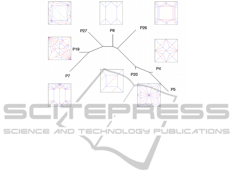
Figure 2: The pilot set with just E
1
, with the BioNJ filter.
With the UP weight some clustering of similar pairs
can be seen with UPGMA, as shown in Figure 4. In
the pilot set it appears that the UP weight is a better
indicator of similarity than the Bio weight, suggesting
that V
1
and E
3
are rather deficient as features for mea-
suring the perceptual similarity of geometric graphs.
Figures 3 and 4 show that both the UP and the
BIO weights display similar clustering with some of
the patterns, such as (33, 35), (36, 37), and (25, 31).
However, while the two are not always in agreement
with respect to which pairs are most similar, they gen-
erally agree on two that are very distant from each
other.
5 CONCLUSION AND FUTURE
DIRECTIONS
The present preliminary study provides sufficient mo-
tivation to perform an experiment with a group of hu-
man subjects to determine more objectively how well
our measure of geometric graph similarity correlates
with human judgments of the similarity of origami
crease patterns. Furthermore, it would be then be
interesting to determine if generalizing the distance
measure tested here to computing minimum-weight
many-to-many matchings would offer any improve-
ment over using perfect matchings. It is also planned
to compare the measure tested here with other mea-
sures of geometric graph similarity. In particular,
computing the many-to-many optimal matching for
certain one-dimensional strings is computationally
more efficient that the Hungarian algorithm for two-
dimensional geometric graphs (Eiter and Mannila,
1997), (Colannino et al., 2007), (Mohamad et al.,
2014). Hence it is worth determining the viabil-
ity of converting CPs to one-dimensional strings that
can be tackled with one-dimensional many-to-many
techniques. In addition we would like to determine
whether there is any correlation between the similar-
ity of the crease patterns and the similarity of their
respective folded objects. Crease patterns have also
found application to the documentation of origami
(Lang, 2012), (Akitaya et al., 2013). Therefore, it
will be explored how the phylogenetic trees computed
from collections of crease patterns can contribute to
this documentation, as well as inform the historical
evolution of origami designs.
ACKNOWLEDGEMENTS
The authors are grateful to the reviewers for useful
suggestions, and to the High Performance Computing
resource center of New York University Abu Dhabi
for making their super-computer BuTinah available
for the experiments.
REFERENCES
Akitaya, H. A., Mitani, J., Kanamori, and Fukui, Y. (2013).
Generating folding sequences from crease patterns of
flat-foldable origami. In Proceedings of the Special
Interest Group on Graphics, pages 991–1000. ACM.
Ambauen, R., Fischer, S., and Bunke, H. (2003). Graph edit
distance with node splitting and merging, and its ap-
ICPRAM2015-InternationalConferenceonPatternRecognitionApplicationsandMethods
390

plication to diatom idenfication. In Proc. 4th IAPR
Intl. Conf. Graph Based Representations in Pattern
Recognition, pages 95–106.
Arkin, E. M., Bender, M. A., Demaine, E. D., Demaine,
M. L., Mitchell, J. S. B., Sethia, S., and Skiena, S. S.
(2004). When can you fold a map? Computational
Geometry: Theory and Applications, 29(1):166–195.
Balkom, D. J., Demaine, E. D., and Demaine, M. L. (2004).
Folding paper shopping bags. In Proceedings of the
14th Annual Fall Workshop on Computational Geom-
etry, pages 14–15. MIT, Cambridge.
Bern, M. and Hayes, B. (1996). The complexity of flat
origami. In Proceedings of the 7th Annual ACM-SIAM
Symposium on Discrete Algorithms, pages 175–183,
Atlanta.
Berretti, S., Del Bimbo, A., and Pala, P. (2004). A graph edit
distance based on node merging. In Proceedings of the
ACM International Conference on Image and Video
Retrieval (CIVR), pages 464–472, Dublin, Ireland.
Cheong, O., Gudmundsson, J., Kim, H.-S., Schymura, D.,
and Stehn, F. (2009). Measuring the similarity of ge-
ometric graphs. In Experimental Algorithms, pages
101–112. Springer.
Clapper, B. (2008). Munkres algorithm for the assignment
problem ver.1.0.6.
Colannino, J., Damian, M., Hurtado, F., Langerman, S.,
Meijer, H., Ramaswami, S., Souvaine, D., and Tou-
ssaint, G. T. (2007). Efficient many-to-many point
matching in one dimension. Graphs and Combina-
torics, 23:169–178.
Demaine, E. and O’Rourke, J. (2007). Geometric Fold-
ing Algorithms: Linkages, Origami, Polyhedra. Cam-
bridge University Press, New York.
Demaine, E. D. and Demaine, M. L. (2001). Recent results
in computational origami. In Origami
3
: Proc. of the
3rd International Meeting of Origami Science, Math,
and Education, pages 3–16, Monterey, California.
Eiter, T. and Mannila, H. (1997). Distance measures for
point sets and their computation. Acta Informatica,
34(2):109–133.
Fei, H. and Huan, J. (2008). Structure feature selection
for graph classification. In Proceedings of the 17th
ACM conference on Information and knowledge man-
agement, pages 991–1000. ACM.
Gao, X., Xiao, B., and Tao, D. (2010). A survey of
graph edit distance. Pattern Analysis and Applica-
tions, 13:113–129.
Gascuel, O. (1997). Bionj: an improved version of the nj
algorithm based on a simple model of sequence data.
Molecular biology and evolution, 14(7):685–695.
Graham, R. L. (1987). A similarity measure for graphs. Los
Alamos Science, pages 114–121.
Gu, C. and Guibas, L. (2011). Distance between folded
objects. In Proceedings of the European Workshop on
Computational Geometry, pages 40–42.
Hodge, T., Jamie, M., and Cope, T. (2000). A myosin family
tree. Journal of Cell Science, 113(19):3353–3354.
Huson, D. H. and Bryant, D. (2006). Application of phylo-
genetic networks in evolutionary studies. Molecular
biology and evolution, 23(2):254–267.
Kuhn, H. W. (1955). The hungarian method for the assign-
ment problem. Naval Research Logistics Quarterly,
2(1-2):83–97.
Lang, R. J. (1996). A computational algorithm for origami
design. In Proceedings of the Twelfth Annual Sym-
posium on Computational Geometry, SCG ’96, pages
98–105, New York, NY, USA. ACM.
Lang, R. J. (2012). Origami Design Secrets: Mathematical
Methods for an Ancient Art. CRC Press.
Levenshtein, V. I. (1966). Binary codes capable of correct-
ing deletions, insertions, and reversals. Soviet Physics
Doklady, 10(8):707–710.
Liapi, K. A. (2002). Transformable architecture inspired
by the origami art: Computer visualization as a tool
for form exploration. In Proceedings of the 2002
Annual Conference of the Association for Computer
Aided Design In Architecture, pages 381–388.
McArthur, M. and Lang, R. J. (2013). Folding Paper: The
Infinite Possibilities of Origami. Tuttle Publishing,
Hong Kong.
Mitani, J. (2011). Oripa origami pattern editor.
http://mitani.cs.tsukuba.ac.jp/oripa.
Mohamad, M., Rappaport, D., and Toussaint, G. T. (2014).
Minimum many-to-many matchings for computing
the distance between two sequences. Graphs and
Combinatorics.
Munkres, J. (1957). Algorithms for the assignment and
transportation problems. Journal of the Society of In-
dustrial and Applied Mathematics, 5(1):32–38.
O’Rourke, J. (2011). How to Fold It: The Mathematics of
Linkages, Origami and Polyhedra. Cambridge Uni-
versity Press, New York.
Pach, J. (2004). Towards a Theory of Geometric Graphs.
No. 342. American Mathematical Society.
Post, O. and Toussaint, G. T. (2011). The edit distance as a
measure of perceived rhythmic similarity. Empirical
Musicology Review, 6(3):164–179.
Robles-Kelly, A. and Hancock, E. R. (2005). Graph edit dis-
tance from spectral seriation. IEEE Trans. on Pattern
Analysis and Machine Intelligence, 27(3):365–378.
Tachi, T. (2010). Rigid-foldable structure using bidirection-
ally flat-foldable planar quadrilateral mesh. In Ad-
vances in Architectural Geometry, pages 87–102.
Wu, W. and You, Z. (2011). A solution for folding rigid tall
shopping bags. Proceedings of the Royal Society – A,
pages 1–14.
ADissimilarityMeasureforComparingOrigamiCreasePatterns
391

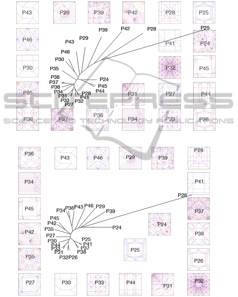
Appendix
Figure 3: The half set with the Bio weights, using the UPGMA filter.
Figure 4: The half set with the UP weight, using the UPGMA filter.
ICPRAM2015-InternationalConferenceonPatternRecognitionApplicationsandMethods
392

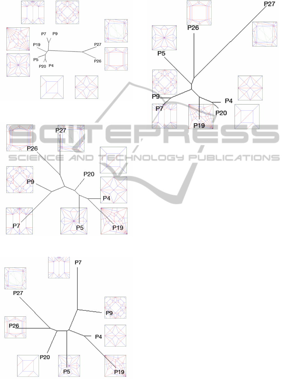
Figure 5: The pilot set with the UP weights, using the UP-
GMA filter.
Figure 6: The pilot set with the UP weights, using the BioNJ
filter.
Figure 7: The pilot set with the Bio weights, using the
BioNJ filter.
Figure 8: The pilot set with the Bio weights, using the UP-
GMA filter.
ADissimilarityMeasureforComparingOrigamiCreasePatterns
393