
Inverse Light Design for High-occlusion Environments
Anastasios Gkaravelis, Georgios Papaioannou and Konstantinos Kalampokis
Department of Informatics, Athens University of Economics and Business, Athens, Greece
Keywords:
Computer Graphics, Light Design, Optimization, Inverse Light Positioning Problem.
Abstract:
Lighting design is a demanding but very important task in computer cinematography, games and architectural
design. Computer-assisted lighting design aims at providing the designers with tools to describe the desired
outcome and derive a suitable lighting configuration to match their goal. In this paper, we present an automatic
approach to the inverse light source emittance and positioning problem, based on a layered linear / non-linear
optimization strategy and the introduction of a special light source indexing according to the compatibility
of each individual luminary position with the desired illumination. Our approach is independent of a partic-
ular light transport model and can quickly converge to an appropriate and plausible light configuration that
approximates the desired illumination and can handle environments with high occlusion.
1 INTRODUCTION
Lighting design is a very important task in order to
correctly illuminate a scene, emphasizing individual
aspects of the scene or establishing a specific mood. It
plays an essential role, especially in the entertainment
industry, and more specifically in computer cine-
matographyand games. Also, it is a necessary process
in architectural modelling, where energy-efficientand
well-balanced illumination from artificial luminaries
needs to be carefully devised. Despite its importance,
lighting design is also a tedious and - more often than
not - a counter-intuitive procedure. To manually il-
luminate a scene, the artist has to carefully and iter-
atively adjust the lighting parameters in a trial-and-
error basis, until the desired effect is achieved. Thus,
automatic methods have emerged, which compute the
lighting parameters to achieve a user-specified light-
ing result, requiring minimal or even no manual inter-
vention.
Due to the nature of light transport in an arbitrary
environment, the generalized inverse lighting prob-
lem is a very complex one to solve. Therefore, as
mentioned in (Patow and Pueyo, 2003), it is often
partitioned into sub-problems, such as the light emit-
tance problem (EP) and the light source positioning
(LSP) problem. First attempts only solved a simpler,
more tightly-constrained problem, such as the indi-
rect light adjustment via shadow manipulation (e.g.
(Poulin and Fournier, 1992), (Poulin et al., 1997)).
As researchers got more comfortable with the inverse
lighting problem, unified emittance/positioning solu-
tions were sought. Despite the progress in this field,
the inverse lighting problem is still challenging and
it becomes increasingly more complex due to the de-
mand for increased realism by including global illu-
mination in the inverse lighting calculations and the
ability to handle dynamic environments.
In this paper, we present an algorithm that, given
a number of lights and the desired illumination, com-
putes their position and emittance by using optimiza-
tion techniques and heuristics to guide them (see ex-
ample in Figure 1). As usual, we describe the de-
sired illumination by using an irradiance goal at user-
specified sample locations, although any goal can be
used, such as a uniform lighting level across random
locations distributed within the environment.
Our inverse lighting algorithm consists of three
major steps. In the first step, we discretize the param-
eter space of the possible light source positions into
a grid of cells and compute an emittance-independent
contribution or coverage of these potential light posi-
tions to the sampling points. We build a special index
that allows querying light positions based on a spe-
cific sampling point coverage pattern. We exploit this
index to efficiently find the globally optimal combina-
tion of cells (coarse light positions) and emittance that
match the lighting goal, using Simulated Annealing
with an inner linear optimizer for the emittance. Fi-
nally, we deploy a non-linear optimization algorithm
to fine-tune the light source positions in order to over-
come the discretization simplification.
26
Gkaravelis A., Papaioannou G. and Kalampokis K..
Inverse Light Design for High-occlusion Environments.
DOI: 10.5220/0005291400260034
In Proceedings of the 10th International Conference on Computer Graphics Theory and Applications (GRAPP-2015), pages 26-34
ISBN: 978-989-758-087-1
Copyright
c
2015 SCITEPRESS (Science and Technology Publications, Lda.)
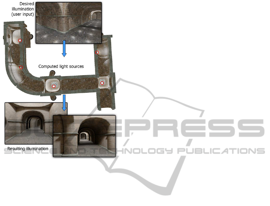
Figure 1: Inverse lighting pipeline, using the proposed
method.
The main contributions of this paper are:
• A novel indexing of light configurations based on
their contribution to the specified goal (coverage).
This index allows fast queries of alternative light
positions to satisfy a particular goal, correspond-
ing to a clustering in coverage space.
• A robust mapping of the EP/LSP problem to the
Simulated Annealing optimization method and a
respective practical algorithm using the light cov-
erage indexing.
The remainder of the paper is organized as fol-
lows. Section 2 places our method in the context of
the related work. Sections 3 and 4 provide a formu-
lation for our coverage-space solving strategy and a
description of the process. Section 5 presents com-
parative results and discusses the performance of our
method. Finally, in Section 6 we present our conclu-
sions and future research directions.
2 PREVIOUS WORK
For the inverse lighting problem, several methods
have been proposed. Similar to (Patow and Pueyo,
2003), here we partition the inverse lighting problem
into sub-problems and briefly present some represen-
tative techniques and applications from each category.
For a more comprehensive, recent survey of the field,
please refer to (Schmidt et al., 2014). Furthermore, at
the end of this section we provide more details on a
recent method that we compare our work with.
Light Source Emittance Problem. (Schoeneman
et al., 1993) proposed a method, in which the user
paints the desired illumination on a scene and the in-
tensity of a set of lights with known positions is de-
termined by a constrained least squares solver. The
method relied on the observation that the resulting
lighting on any surface location is a linear combina-
tion of the emittance levels of light sources, provided
the latter remain fixed in space. A similar approach
was implemented by (Anrys et al., 2004) in order to
compute the intensity of a set of light sources by us-
ing and optimizing the luminance of real luminaries,
which were previously set up and their illumination
on a physical object captured in a set of photographs.
(Kawai et al., 1993) performed an optimization
over the intensities and directions of a set of lights as
well as the reflectivity of surfaces in order to best con-
vey the subjective impression of certain scene quali-
ties as expressed by the user and minimize the global
energy of the scene.
(Okabe et al., 2007) presented an algorithm to
manipulate and alter environment maps by directly
painting the outgoing radiance on the target model.
They used a constrained linear least square solver,
which minimizes the weighted squared difference of
the computed and desired illumination. It could han-
dle diffuse and specular reflections and relied on
the SRBF-based Precomputed Radiance Transfer ap-
proach to perform the computations interactively.
Light Source Positioning. (Poulin and Fournier,
1992) proposed a way to define light positions in
a scene by manipulating their shadows or resulting
highlights on both diffuse and specular surfaces. By
selecting a pair of points in a scene, they define the
illumination constraints, which are subsequently used
to position the light source accordingly. Later, (Poulin
et al., 1997) presented a system that controls the posi-
tion of a number of light sources by sketching strokes
where the shadow of selected objects should fall in
a scene. The proposed solution could also provide
feedback regarding the plausibility of a newly placed
stroke. To avoid solving the problem analytically, a
non-linear constraint optimization algorithm was uti-
lized. (Pellacini et al., 2002) developed a user in-
terface system that facilitated the design of shadows.
The shadows in the scene could be selected, trans-
formed or new ”fake” shadows could be introduced.
Inverse Lighting addresses both the emittance and
InverseLightDesignforHigh-occlusionEnvironments
27

positioning of light sources in a unified manner and
several architectures and systems havebeen proposed.
(Costa et al., 1999) introduced an IL system where a
custom scripting language was used to define the illu-
mination constraints. The system utilized the Adap-
tive Simulated Annealing algorithm to optimize the
light sources. (Pellacini et al., 2007) proposed a work-
flow, where artists could directly paint the desired
lighting effects onto the geometry. With the use of
an importance map, obtained from the painted target
image, the system applies the non-linear simplex al-
gorithm (Nelder and Mead, 1965) to adjust the var-
ious parameters of the light sources by minimizing
the goal function, which is a weighted average of the
difference between the desired and computed illumi-
nation.
(Castro et al., 2009) solve the problem of light
positioning and emittance, while keeping the total
emission power at a minimum. They computed the
contribution of a user-defined number of lights using
the radiosity algorithm and experimented with local
search algorithms, such as Hill Climbing and Beam
Search. As a goal, they tried to minimize total emis-
sion power. Later, (Castro et al., 2012) improved the
algorithm and used global approaches to solve the
problem in order to avoid getting stuck in a local op-
timum. They offered an implementation and experi-
mented with Genetic algorithms, Particle Swarm op-
timization and a hybrid combination of a global and
local search algorithm.
An interesting formulation of the ”opening” prob-
lem was suggested by (Fern´andez and Besuievsky,
2012), where skylights were treated as area light
sources and a unified skylight/luminaries optimiza-
tion was sought. They used the VNS metaheuristic
algorithm to solve the inverse lighting problem, while
keeping the energy consumption of the artificial light
sources to a minimum and/or maximize the contribu-
tion of the skylights.
Finally, (Lin et al., 2013) proposed a coarse-to-
fine strategy to solve the inverse lighting problem,
given a set of user-painted lighting samples on sur-
faces. They spread unit-intensity lights in a volume
grid and configure their intensities using a constrained
linear least square solver. Dim lights are pruned and
the process is repeated with the remaining cells, after
subdividing them. Then, a light hierarchy is built and
traversed to obtain a good configuration, which is sub-
sequently optimized using a non-linear least squares
method. Since this is the most recent method, closely
related to ours, in the remainder of the paper, we often
provide direct comparisons with it.
3 PROBLEM FORMULATION
Let I
goal
be an illumination goal over a scene and
P be a light configuration consisting of k lights that
illuminates a scene producing an illumination result
I
res
(P). I
goal
, I
res
can be radiance, radiosity or irradi-
ance, depending on the measurement demands of the
underlying application (e.g. dependence on viewing
direction, material etc.). For a discrete set of surface
samples in the scene s
i
, I
res
(P, s
i
) and I
goal
(s
i
) are the
resulting illumination from the lighting configuration
P and the desired illumination at s
i
, respectively.
Using the above notations, an inverse lighting
problem can be defined as the search for the optimal
lighting configuration P
∗
, which minimizes some dis-
tance function D between the resulting and the desired
illumination at the sampling locations s
i
:
P
∗
= argmin
P
D(I
res
(P, s
i
), I
goal
(s
i
)) (1)
Typically, D is expressed as the L
2
norm of the
measurement differences at all N
s
sampling points s
i
.
For real luminaries, although the dependence of
the emittance L
e
on direction or power consumption
cannot be considered linear, its dependence on a nom-
inal unit output power distribution can: L
e
(l
j
, ω) =
c(l
j
)
˜
L
e
(l
j
, ω). In other words, the measured contribu-
tion of a light source l
j
to the illumination of a given
point is linearly dependent on its emittance scaling
c(l
j
). Therefore, the illumination from a set of n light
sources to a sampling point s
i
is the superposition of
all luminary contributions.
If we consider a general light transport operator
(path integral) LT(l
j
→ s
i
) to describe the total con-
tribution of each light source l
j
to a sampling point s
i
,
for n unit light sources, the lighting result on s
i
is the
linear combination of these contributions with coeffi-
cients c(l
j
).
Assuming now fixed positions for n light sources
covering a discretization of the 3D environment, the
(discrete) LSP and EP problems can be solved simul-
taneously, by optimizing the emittance scaling factors
c(l
j
) of all n potential candidate lights so that the re-
sulting light configuration P
∗
satisfies Equation 1. A
zero c(l
j
) implies the absence of a light source at l
j
.
4 METHOD OVERVIEW
(Lin et al., 2013) solve a simplified version of the
above problem by regarding all potential light sources
positioned on a discretized grid covering the entire
scene and solving a linear system of N
s
equations and
N
c
unknowns, N
s
being the number of light (goal)
GRAPP2015-InternationalConferenceonComputerGraphicsTheoryandApplications
28
sample points and N
c
the number of grid cells, i.e. po-
tential light positions. They evaluate the light contri-
bution using rasterization and solve the linear system
with a least squares method.
In order to make the light optimization problem
manageable, they use a hierarchical (coarse to fine)
solving strategy, starting from a very rough initial dis-
cretization of the scene volume. The calculated emit-
tance scaling factors are clamped and the cells of non-
zero light intensity are further subdivided. The result-
ing lights are clustered in a light tree, whose graph
cut that satisfies an error margin, is refined using a
non-linear optimization method to provide the final
lighting configuration. However, this strategy leads
to solutions that are unsuitable for environments with
dense geometry or heavy occlusion (e.g. typical ar-
chitectural spaces) since the sparsity of the initial po-
tential light locations results in single cells frequently
containing occluders, thus clustering potential lights
near walls, after the cell subdivision, or worse, plac-
ing lights only in one side of the barrier.
Since we needed to overcome this problem, we
strived for a solution that allows a finer initial sub-
division of the space into cells. Solving the inverse
light problem using a linear system, would require a
set of N
s
equations with 3 × N
c
unknowns c
j
(RGB
coefficients), N
c
being the number of cells (potential
lights) and N
s
being the number of sampling points,
where the desired illumination is given. 3 × N
c
can
reach several hundreds of thousands in some expan-
sive scenes and the problem can become practically
intractable. Additionally, to find a stable and usable
solution would require defining a large number of
sampling points, proportional to N
c
, which is imprac-
tical for all purposes. We exploit a discretized ini-
tial light placement, too, but propose a non-linear ap-
proach to light positioning with an inner linear solver
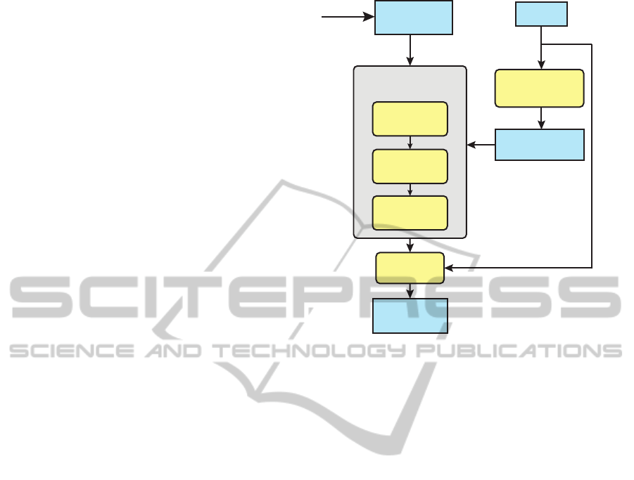
for the emittance adjustment (Figure 2), as follows.
4.1 Light Coverage Computation
We first initialize a set of potential light source posi-
tions on a fine grid (e.g. in the order of 64
3
cells or
more), the center of each cell l
j
representing a po-
tential light source. For each light and each sam-
pling point, we compute the light transport function
LT(l
j
→ s
i
), normalize it over all N
s
sampling points
and store the values as an (3 × N
s
)-dimensional at-
tribute vector f
j
(LT is a three-channel quantity).
Normalizing the attribute vector f
j
transforms the
EP/LSP to a sample coverage problem, because we do
not include the magnitude of the light’s contribution
to the sampling points but rather their ”reachability”
by a given source.
Scene
Goal
Illumination
Light Coverage
Computation
User
Input
Coarse-level
Optimization Loop
Candidate
Selection
Optimize
Emittance
Compute
Error
Final
Configuration
Light Coverage
Index
Refinement
Step
Figure 2: Our algorithm consists of an initialization step,
the main optimization strategy and a final refinement step.
Given as input the goal illumination, our algorithm finds a
lighting configuration that satisfies the goal illumination.
In our current system, to estimate the path integral
LT(l
j
→ s
i
) for all light-sampling point paths, we use
bidirectional path tracing (BPT). This way, we avoid
rasterization problems, such as artifacts introduced by
shadow maps, and we can inherently include complex
global light transport phenomena. However, any path
integral estimator can be utilized instead. For this pa-
per, we use an NVIDIA Optix-based BPT implemen-
tation to compute all light position - sampling point
path integrals in parallel, with a Monte Carlo solver
and 20-100 samples per (l
j
, s
i
) pair.
An important novel step of our approach is that
the light attribute vectors are all together stored in a
k-d tree indexed by attribute vector dimension, i.e.
the structure is a (3× N
s
)-d tree. The normalized at-
tribute vector f
j
allows for a fast search of light posi-
tions with similar sample point coverage. We use the
Nanoflann k-d data structure implementation that al-
lows very fast queries using the Approximate Nearest
Neighbors algorithm. We show next how we exploit
this propertyto performmeaningful mutations of light
configurations P.
4.2 Coarse-level Optimization
To find a light configuration P of k sources that mini-
mizes the distance function D(I
res
(P, s
i
), I
goal
(s
i
)), we
use a non-linear optimization algorithm and in par-
InverseLightDesignforHigh-occlusionEnvironments
29
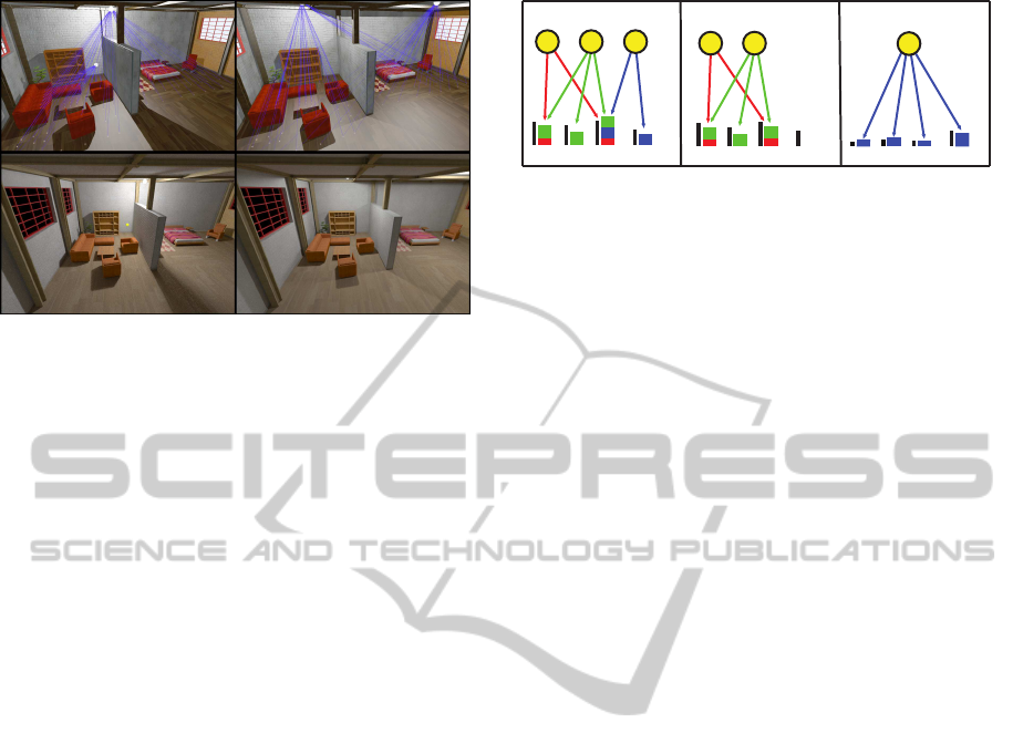
Figure 3: Method comparison - Studio scene. Left: results
from the method by (Lin et al., 2013). Right: our method
optimizes goal point coverage (global path throughput) and
results in more acceptable solutions with better light cover-
age. The preview on the top row shows the direct paths to
the sample (goal) points. The bottom row shows the path-
traced results of the two light configurations.
ticular, Simulated Annealing, with random mutations
over a k-dimensional state vector equal to the cur-
rent choice of light positions. The reason for uti-
lizing a non-linear solver is that although the com-
bined EP/LSP is linear with respect to light contri-
butions, we want to rapidly investigate solutions in
sample coverage space, a non-linear domain and ex-
ploit the fact that light sources in completely different
locations may indeed provide similar coverage to the
sampling points, thus explore seemingly disjoint, al-
beit increasingly favourable solutions.
Separating the coverage problem from the light
source emittance has the additional benefit of produc-
ing more usable solutions, regardless of the explicit
goals provided by the user. For example, in Figure 3
both our method and the method by (Lin et al., 2013),
produce visually similar irradiance near the goal po-
sitions. However, due to better coverage, our method
reduces shadowing, as it better handles occlusion.
Mutation Strategy. For a given light configuration,
we select and remove one light source at random. The
remaining k − 1 lights, constitute an incomplete light
configuration P
(k−1)
for which we compute the con-
tribution I
res
(P
(k−1)
, s
i
) to the N
s
sampling points (see
Emittance Estimation below).
Next, the residual I
goal
(s
i
) − I
res
(P
(k−1)
, s
i
)) is
computed and the resulting normalized attribute vec-
tor f
dif f
is used to locate a number of light sources
with similar attributes in the k-d tree. Simply put,
we use the normalized lighting residual from remov-
ing a light source to locate other source positions
that would better complement the remaining lights in
achieving the goal.
Figure 4: The mutation strategy. After the removal of one
light source (middle), we compute the optimal emittance of
the remaining light sources and estimate the residual illu-
mination that is required to match the goal illumination at
all points. Finally, we locate a light that better matches this
residual (right).
Given the resulting set of nearest lights (in terms
of coverage complementarity, i.e. attribute vector
f
dif f
), we pick one candidate location at random and
replace the missing light source, in order to gener-
ate a new improved light configuration P. The opti-
mal emittance for this new configuration is estimated
and the resulting evaluation of D(I
res
(P, s
i
), I
goal
(s
i
))
is the outcome of the cost function. The entire muta-
tion procedure is illustrated in Figure 4.
When the SA algorithm accepts mutations with a
potentially higher cost, a random mutation of the state
P occurs and the above mutation strategy is omitted.
Emittance Estimation. According to the preceding
discussion, we have decoupled the light position se-
lection strategy from the emittance problem, by esti-
mating the intensities L(l
j
) of a configuration P (i.e.
a set of k fixed light sources) within each position op-
timization step. This is a linear system (Schoeneman
et al., 1993) with only a few unknowns (3× k), which
can be rapidly solved, especially since all F(s
i
, l
j
)
path integrals have been estimated.
For our implementation we chose a non-negative
linear least square solver (Lawson and Hanson, 1987)
since the intensity of a light source could not have a
negative value.
The use of this hybrid non-linear / linear strategy
has a significant impact on convergence, especially
when coupled with our light coverage prioritization
strategy (see evaluation in Section 5).
4.3 Solution Refinement
Similar to (Lin et al., 2013), to find the final, non-
discretized positions of the light sources and their re-
spective emittance, we refine further the light config-
uration solution of the coarse-level optimization. This
is achieved by again running a hybrid non-linear / lin-
ear optimizer, only this time, the light - sample path
integrals need to be evaluated in each optimization it-
eration, although for only k light sources. Based on
GRAPP2015-InternationalConferenceonComputerGraphicsTheoryandApplications
30
0 50 100 150 200 250
35%
37%
33%
31%
29%
27%
25%
Error
Iterations
Renement Stage Convergence
Hybrid
Non-linear
Figure 5: Convergence rate of the refinement stage using a
position/emittance non-linear optimization versus a hybrid
linear (emittance) / non-linear (position) strategy.
our experiments and the suggestion in (Pellacini et al.,
2007) and (Lin et al., 2013), as a non-linear optimizer
we use the nonlinear simplex algorithm (Nelder and
Mead, 1965), which performsvery well given that it is
initialized with an already near-optimal solution. The
parameter space of the non-linear optimizer (i.e. the
light positions) is very narrow, since the light posi-
tions only need to be jittered by at most the size of
one cell.
Again, after estimating the path integrals in each
iteration, we employ the non-negative linear least
square solver to adjust the emittance of the given light
configuration.
Figure 5 demonstrates the faster convergence of
the hybrid algorithm when compared to a unified non-
linear optimization algorithm (non-linear simplex in
this case) to simultaneously optimize position as well
as source emittance.
5 EVALUATION AND RESULTS
We tested our method on scenes of varying geomet-
ric complexity. We mainly focused on environments
that have a high degree of shape and structure com-
plexity such as scenes consisting of separate regions
with high occlusion, since such complex scenes are
commonly found on cinematic imagery, games or ar-
chitectural designs. The tests were performed on an
Intel i7-4930 CPU and a Nvidia Geforce GTX 780
and we report times in seconds. The CPU side of
the algorithm was ran in a single thread without tak-
ing advantage of multi-core CPUs, although it can be
very easily parallelized to take advantage of multi-
threading systems by running concurrent instances of
the SA method or splitting the search space. In our
tests, we used 1000 iterations for the Simulated An-
nealing process, which were sufficient since by us-
ing our mutation strategy and the fast clustered search
mechanism (via the coverage index), we were able to
obtain a good solution in only a few iterations.
Correctness. First, we evaluated the accuracy of our
Figure 6: Correctness experiment. Left: the user defined
light sources, whose irradiance to sampling points is mea-
sured and used as a goal. Right: the computed light config-
uration produced by our algorithm (4.3% error).
method: We illuminated a scene with a known light-
ing configuration and tried to re-establish the same
lighting configuration by using our algorithm. The
scene we used was the Apartment environmentof Fig-
ure 6 that has 8 rooms and a hallway connecting them.
We manually placed 10 light sources at typical loca-
tions inside the scene and computed their contribu-
tion at random sampling positions s
i
(Figure 6 (left)).
Then, we ran our method using the computed con-
tribution as the goal illumination I
goal
(s
i
). The com-
puted luminaries (Figure 6 (right)) were very close to
the manual configuration. It took our algorithm 40
seconds to compute the result and the normalized il-
lumination difference between the goal and resulting
illumination was 4.3%.
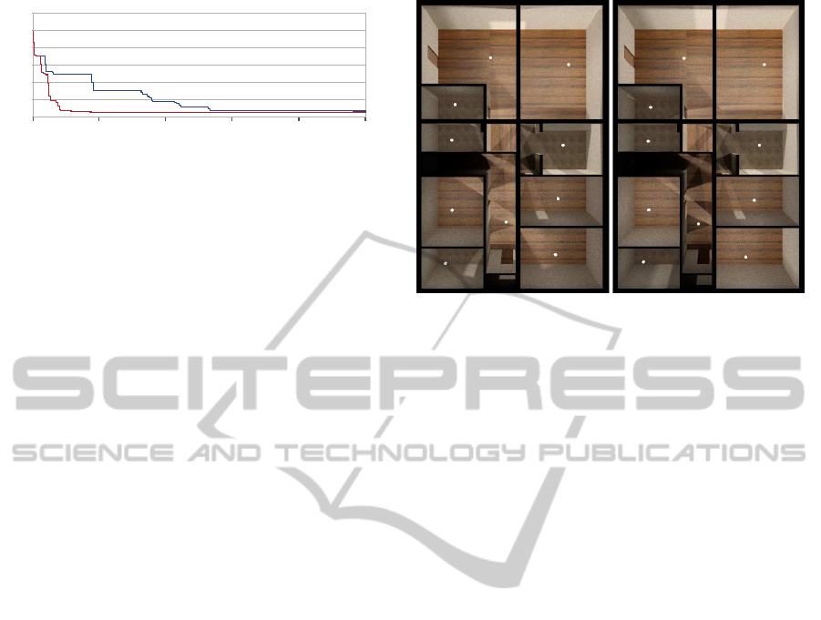
Mutation Strategy. We tested the convergence rate
of our light configuration mutation strategy against
the random selection approach. We confirmed that re-
placing one of the k light sources with one that com-
plements the missing contribution to the sampling
points ensures a significantly faster convergence to a
better solution than in the case of randomly select-
ing a new light source (Figure 7). Even if we choose
more iterations for the random selection method, it
is evident that the complementary coverage approach
always results in a better solution, due to its prioriti-
zation of regions that are inadequately illuminated.
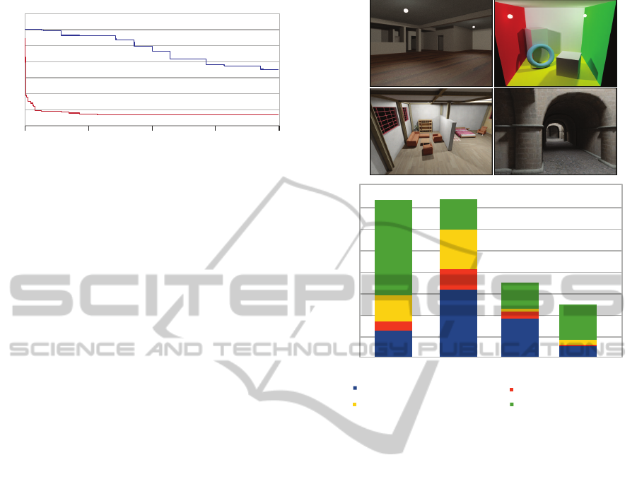
Performance. In Figure 8 we measure and present
the performance of the stages of our algorithm. We
selected various scenes with different structural com-
plexity (high or low occlusion) and polygon count.
We measured the initialization step, where we com-
pute the coverage of the light sources, the index con-
struction, the Coarse-Level optimization and the final
InverseLightDesignforHigh-occlusionEnvironments
31
0 700 1400 2100 2800
60%
50%
40%
30%
20%
10%
Error
Iterations
Our mutation strategy
Random state selection
SA Convergence
Figure 7: Convergence rate of the coarse-level optimization
stage (simulated annealing) using standard state transitions
and our mutation strategy.
solution refinement step.
Figure 8 confirms that the initialization time de-
pends on the polygon count of the scene, since we
need to compute the coverage of every light source,
which involves tracing paths within a larger environ-
ment. In every scene we compute the global illumina-
tion of the light sources, except from the Sewers scene
where we only used direct illumination. It is obvious
that by only using direct illumination, the computa-
tion of the illumination is greatly reduced.
On the other hand, the Coarse-Level optimization
step does not depend on the polygon count of the
scene, since the light coverage of every light source
is already computed, but on the structural complexity
of the scene and the feasibility of the desired illumi-
nation. One example is the Studio scene where, given
a configuration of two lights, there are many possible
light configurations that satisfy our goal, thus the op-
timizer takes more time to converge to a global opti-
mum. Another example is the Sewers scene, which is
a scene with high occlusion. However, the algorithm
can easily mark regions that need to be covered and
place light sources in positions that minimize the cost
function, locating a good configuration very quickly.
Finally, the refinement step does not only depend
on the polygon count of the scene, since we need
to compute the illumination of the evaluated con-
figuration at every step, but it is also affected by
how close the current solution is to the optimal one.
Even though the Studio scene has the highest poly-
gon count, the solution refinement step found a solu-
tion very quickly, because the configuration from the
Coarse-Level Optimization step was very close to the
optimal solution. On the other hand, the refinement
step took more time on the Apartment scene, since
there were more light sources to optimize, coupled
with the fact that small state changes of the light posi-
tions can significantly alter the resulting illumination
due to high occlusion.
Comparative Evaluation. Below we compare our
Apartment Studio Cornell Sewers
0
5
10
15
20
25
30
35
40
Solution Refinement
Initialization
Index Construction
Coarse-Level Optimization
Time (Seconds)
Scenes
Apartment
Studio
Cornell
Sewers
Figure 8: Perfomance measurements of the various stages
of the algorithm with simple and complex scenes.
algorithm with the recently published lighting opti-
mization method of (Lin et al., 2013). We compare
their performance using complex environments with
high occlusion. First, we test both methods with the
Apartment scene, which has separate regions with
high occlusion. As a goal, in both experiments we
used the illumination produced by a known initial
light configuration (see Correctness paragraph).
As we previously mentioned, our method per-
forms quite well for a configuration of 10 lights, with
the normalized illumination difference to the desired
illumination being at 4.3%. In order to check the ro-
bustness of our algorithm, we tried to satisfy the illu-
mination goal by using fewer light sources. We chose
8 light sources since the scene has 8 separate rooms
(connected via a doorway to others). Figure 9 shows
a comparison of the two methods. On the right, we
show the results from our implementation with a nor-
malized illumination difference of 12%. In the left
inset, we present the lighting configuration that the al-
gorithm by (Lin et al., 2013) found for an 8-light con-
figuration, producing a normalized illumination dif-
ference of 36.7% in 35 seconds. The method by (Lin
et al., 2013) failed to compute the correct light con-
figuration, resulting in luminaries with high error and
failure to include lights in certain spaces, because of
GRAPP2015-InternationalConferenceonComputerGraphicsTheoryandApplications
32

Figure 9: Lighting configuration comparison - Apartment
scene. Left: the compared method. Right: our method.
The line segments represent the path throughput of domi-
nant path integrals (green: high, blue: low).
its hierarchical light placement strategy. A hierarchi-
cal (coarse-to-fine) scheme fails, if the coarse can-
didate solutions cannot successfully represent their
neighborhood. In this case, large cells intersect the
boundaries of separate spaces and result in biased
placement of luminaries. In some scenes, a finer grid
can be used, but this does not alleviate the problem,
unless the boundaries of the cells roughly coincide
with the occluding structures. Also, another problem
of using a finer grid is that the linear least squares
solver tries to optimize lights that are near the sam-
pling points in order to minimize the error,which does
not work well with the clustering method (light tree),
despite our effort to optimize the parameters and grid
size to give the best results.
Next, we run experiments with the Studio scene
shown in Figure 3, which is a single space featuring
a large occluder and a lot of complex geometry. In
the Studio scene, we defined the goal illumination at
the bedroom and the living room by manually paint-
ing the desired irradiance directly on the geometry
(Figure 3, top row) and then compute the emittance
and position of 2 light sources to satisfy this goal.
Even though, this scene is suitable to be solved with a
coarse-to-fine method, the compared method achieves
a score of 44.5% normalized illumination difference
in 30 seconds, while our method achieves a score of
24.8%.
6 CONCLUSION
We have presented a method to solve the inverse light
positioning / emittance problem, which efficiently
computes the configuration of a given number of light
sources, in order to satisfy the design goals. We pro-
posed a scheme for the efficient representation of can-
didate light configurations to directly search and clus-
ter the light position space according to the light’s
contribution to the desired illumination. This, along
with a hybrid linear / non-linear optimizer that disas-
sociates the emittance and light positioning, lead to a
fast convergence to usable solutions for environments
with high occlusion.
Currently, our system handles only point light
sources, but with no restriction on the materials of
surfaces, while it also provides a user interface for
painting the desired irradiance on any surface. In the
future, we would like to address the problem of deter-
mining the number of lights to be used, by carefully
covering the geometry to be illuminated with the least
amount of light sources that will minimize the error in
a meaningful manner. Furthermore, we would like to
also support area luminaries and include sky lighting
in the calculations, so we can take into consideration
the contribution of natural light, which is very impor-
tant in architectural design.
ACKNOWLEDGEMENTS
This research has been co-financed by the European
Union (European Social Fund - ESF) and Greek na-
tional funds through the Operational Program ”Edu-
cation and Lifelong Learning” of the National Strate-
gic Reference Framework (NSRF) - Research Fund-
ing Program: ARISTEIA II-GLIDE (grant no.3712).
REFERENCES
Anrys, F., Dutr´e, P., and Willems, Y. (2004). Image based
lighting design. In the 4th IASTED International Con-
ference on Visualization, Imaging, and Image Pro-
cessing, page 15.
Castro, F., Acebo, E., and Sbert, M. (2009). Heuristic-
search-based light positioning according to irradiance
intervals. In Proceedings of the 10th International
Symposium on Smart Graphics, SG ’09, pages 128–
139, Berlin, Heidelberg. Springer-Verlag.
Castro, F., del Acebo, E., and Sbert, M. (2012). Energy-
saving light positioning using heuristic search. Eng.
Appl. Artif. Intell., 25(3):566–582.
Costa, A. C., Sousa, A. A., and Ferreira, F. N. (1999). Light-
ing design: A goal based approach using optimisation.
InverseLightDesignforHigh-occlusionEnvironments
33

In Proceedings of the 10th Eurographics Conference
on Rendering, EGWR’99, pages 317–328, Aire-la-
Ville, Switzerland, Switzerland. Eurographics Asso-
ciation.
Fern´andez, E. and Besuievsky, G. (2012). Technical sec-
tion: Inverse lighting design for interior buildings
integrating natural and artificial sources. Comput.
Graph., 36(8):1096–1108.
Kawai, J. K., Painter, J. S., and Cohen, M. F. (1993). Ra-
dioptimization: Goal based rendering. In Proceedings
of the 20th Annual Conference on Computer Graphics
and Interactive Techniques, SIGGRAPH ’93, pages
147–154, New York, NY, USA. ACM.
Lawson, C. and Hanson, R. (1987). Solving Least Squares
Problems. PrenticeHall.
Lin, W.-C., Huang, T.-S., Ho, T.-C., Chen, Y.-T., and
Chuang, J.-H. (2013). Interactive lighting design with
hierarchical light representation. Comput. Graph. Fo-
rum, 32(4):133–142.
Nelder, J. A. and Mead, R. (1965). A simplex method
for function minimization. The computer journal,
7(4):308–313.
Okabe, M., Matsushita, Y., Shen, L., and Igarashi, T.
(2007). Illumination brush: Interactive design of all-
frequency lighting. In Proceedings of the 15th Pacific
Conference on Computer Graphics and Applications,
PG ’07, pages 171–180, Washington, DC, USA. IEEE
Computer Society.
Patow, G. and Pueyo, X. (2003). A survey of inverse render-
ing problems. Computer Graphics Forum, 22(4):663–
687.
Pellacini, F., Battaglia, F., Morley, R. K., and Finkelstein,
A. (2007). Lighting with paint. ACM Trans. Graph.,
26(2).
Pellacini, F., Tole, P., and Greenberg, D. P. (2002). A
user interface for interactive cinematic shadow design.
ACM Trans. Graph., 21(3):563–566.
Poulin, P. and Fournier, A. (1992). Lights from highlights
and shadows. In Proceedings of the 1992 Symposium
on Interactive 3D Graphics, I3D ’92, pages 31–38,
New York, NY, USA. ACM.
Poulin, P., Ratib, K., and Jacques, M. (1997). Sketching
shadows and highlights to position lights. In Proceed-
ings of the 1997 Conference on Computer Graphics
International, CGI ’97, pages 56–, Washington, DC,
USA. IEEE Computer Society.
Schmidt, T.-W., Pellacini, F., Nowrouzezahrai, D., Jarosz,
W., and Dachsbacher, C. (2014). State of the art in
artistic editing of appearance, lighting, and material.
In Eurographics 2014 - State of the Art Reports, Stras-
bourg, France. Eurographics Association.
Schoeneman, C., Dorsey, J., Smits, B., Arvo, J., and Green-
berg, D. (1993). Painting with light. In Proceedings
of the 20th Annual Conference on Computer Graphics
and Interactive Techniques, SIGGRAPH ’93, pages
143–146, New York, NY, USA. ACM.
GRAPP2015-InternationalConferenceonComputerGraphicsTheoryandApplications
34
