
TextTrail
A Robust Text Tracking Algorithm In Wild Environments
Myriam Robert-Seidowsky
1
, Jonathan Fabrizio
1
and S´everine Dubuisson
2
1
LRDE-EPITA, 14-16, rue Voltaire, F-94276, Le Kremlin Bicˆetre, France
2
CNRS, UMR 7222, ISIR, F-75005, Paris, France
Keywords:
Text Tracking, Particle Filter, Likelihood Function, Tangent Distance.
Abstract:
In this paper, we propose TextTrail, a new robust algorithm dedicated to text tracking in uncontrolled envi-
ronments (strong motion of camera and objects, partial occlusions, blur, etc.). It is based on a particle filter
framework whose correction step has been improved. First, we compare some likelihood functions and in-
troduce a new one which integrates tangent distance. We show that this likelihood has a strong influence on
the text tracking performances. Secondly, we compare our tracker with a similar one and finally an example
of application is presented. TextTrail has been tested on real video sequences and has proven its efficiency.
In particular, it can track texts in complex situations starting from only one detection step without needing
another one to reinitialize the model.
1 INTRODUCTION
With the increasing amount of videos, automatic text
extraction has become an essential topic in the com-
puter vision application field. Whereas many works
have already been published on text detection and its
extraction in single images, video context has been
still little investigated. To extend detection process
from an image to a video sequence, a simple way is
to apply a detector on each frame. However, this is
not optimal. First, because the detection process may
be very time consuming, especially for high textured
frames. Secondly, because this “naive” approach does
not provide the matching information between detec-
tions in consecutive frames. However, these associa-
tions are needed for some applications.Visual tracking
algorithms are a solution for such purpose: they at-
tempt to predict the position of text areas at each time
step by using previous information and then provide
some stability of detections or estimations with time.
We could cite a lot of target applications for which
text tracking is important, such as automatic text ex-
traction for indexation, text-to-speech (for example
for visually-impaired persons) or online text transla-
tion (for example for tourists). In these cases, tracking
can improve the final transcription through redundant
information and provides only one transcription per
text area. It can also be fundamental in online text re-
moval: if one specifies a text to erase within a frame, a
removalprocess can be automatically propagated over
the whole sequence by using inpainting algorithms.
Thus, the main goal of text tracking is to collect a list
of associated text regions throughout a sequence by
minimizing the number of detection steps, as this step
can be very time consuming.
State of the art about text tracking is quite re-
stricted. Phan et al. (Phan et al., 2013) used the
Stroke Width Transform to estimate a text mask in
each frame. SIFT descriptors in keypoints from
the mask are extracted and matched between two
frames. Because only text pixels are tracked, it
is robust to background changes but, unfortunately,
only handles static or linear motions. Most of re-
cent approaches (Tanaka and Goto, 2008; Merino and
Mirmehdi, 2007; Minetto et al., 2011) use a particle
filter. Merino et al. (Merino and Mirmehdi, 2007)
proposed a method for text detection and tracking
of outdoor shop signs or indoor notices, that han-
dles both translations and rotations. Here, SIFT de-
scriptors are computed in each component of a de-
tected word (that is supposed to be a letter). Tanaka et
al. (Tanaka and Goto, 2008) suggested two schemes
for signboard tracking: (i) a region-based matching
using RGB colors, and (ii) a block-based matching.
In all prior algorithms, also known as tracking-by-
detection, text is first detected in each frame, then
“tracked” between frames, by using a matching step
that associates detected text areas. However, a recent
algorithm, Snoopertrack (Minetto et al., 2011), de-
268
Robert-Seidowsky M., Fabrizio J. and Dubuisson S..
TextTrail - A Robust Text Tracking Algorithm In Wild Environments.
DOI: 10.5220/0005292002680276
In Proceedings of the 10th International Conference on Computer Vision Theory and Applications (VISAPP-2015), pages 268-276
ISBN: 978-989-758-091-8
Copyright
c
2015 SCITEPRESS (Science and Technology Publications, Lda.)

tects text every 20 frames, and tracks it between them,
using HOGs as feature descriptors.
In this paper, we focus on text tracking. Our al-
gorithm, called TextTrail relies on the particle filter
framework, well known to handle potential erratic and
fast motion. Our tracker is initialized using our pre-
vious work on text localization in single images (Fab-
rizio et al., 2013). This detector is restricted to block
letters text in a Latin alphabet, but could easily be ex-
tended to other alphabet by adapting its learning pro-
cess. Compared to the state of the art, our algorithm
TextTrail can accurately track text regions during a
long time (hundreds of frames) without needing to
reinitialize the model(s) with new detections. We in-
troduce a new likelihood used in the correction step of
the particle filter which uses the tangent distance be-
tween grayscale patches. This likelihood function has
been studied and compared with other ones including
common ones relying on Bhattacharyya distance be-
tween HOG descriptors (Medeiros et al., 2010; Tuong
et al., 2011; Breitenstein et al., 2009). Our tests
show that the tangent distance is really suitable for
text tracking purposes. The paper is organized as fol-
lows. In Section 2 we quickly introduces the particle
filter and the tangent distance. Then, in Section 3, we
expose different likelihoods for text tracking before
proposing a new one (the one we use in TextTrail).
We compare them in Section 4 and evaluate TextTrail
performances. We also compare our approach with a
similar one. In addition we illustrate its interest by
integrating it into a complete scheme of application.
Concluding remarks are finally given in Section 5.
2 BACKGROUND
2.1 Particle Filter
The particle filter (PF) framework (Gordon et al.,
1993) aims at estimating a state sequence {x
t
}
t=1,...,T
,
whose evolution is given, from a set of observations
{y
t
}
t=1,...,T
. From a probabilistic point of view, it
amounts to estimate for any t, p(x
t
|y
1:t
). This can be
computed by iteratively using Eq. (1) and (2), which
are respectively referred to as a prediction step and a
correction step.
p(x
t
|y
1:t−1
) =
R
x
t−1
p(x
t
|x
t−1
)p(x
t−1
|y
1:t−1
)dx
t−1
(1)
p(x
t
|y
1:t
) ∝ p(y
t
|x
t
)p(x
t
|y
1:t−1
) (2)
In this case, p(x
t
|x
t−1
) is the transition and p(y
t
|x
t
)
the likelihood. PF aims at approximating the above
distributions using weighted samples {x
(i)
t
, w
(i)
t
} of N
possible realizations of the state x
(i)
t
called particles.
In its basic scheme, PF first propagates the particle set
{x
(i)
t−1
, w
(i)
t−1
} (Eq. (1)), then corrects particles’ weights
using the likelihood, so that w
(i)
t
∝ p(y
t
|x
(i)
t
), with
∑
N
i=1
w
(i)
t
= 1 (Eq. (2)). The estimation of the pos-
terior density p(x
t
|y
1:t
) is given by
∑
N
i=1
w
(i)
t
δ
x
(i)
t
(x
t
),
where δ
x
(i)
t
are Dirac masses centered on particles x
(i)
t
.
A resampling step can also be performed if necessary.
2.2 Tangent Distance
Tangent Distance (TD) allows to robustly compare
two patterns against small transformations. It was
first introduced by Simard et al. (Simard et al.,
1992) and was mostly used for character recogni-
tion (Schwenk and Milgram, 1996), but also for face
detection and recognition (Mariani, 2002), speech
recognition (Macherey et al., 2001) and motion com-
pensation (Fabrizio et al., 2012).
To compare two patterns I and J, the Euclidean
distance is not efficient as these two patterns may un-
dergo transformations. With TD, a set of potential
transformations is modeled. As these transformations
are not linear, we consider an approximation with lin-
ear surfaces. Here, the Euclidean distance is not com-
puted between the two patterns, but between the two
linear surfaces. Obviously, amplitudes of these trans-
formations are unknown. In our case, we model trans-
formations only on one pattern (in this example J). If
we note d
ec
(., .) the Euclidean distance, the TD is:
min(d
ec
(I, J +
M
∑
i=1
λ
i
V
i
)) (3)
with V
i
the tangent vector of i-th modeled transfor-
mation and λ
i
its contribution. In this minimization
scheme, I and J are known. Tangent vectors can be
computed numerically or analytically. On the con-
trary, all coefficients λ
i
are unknown: the result of the
minimization gives their optimal values.
3 PROPOSED APPROACH
3.1 Framework
We propose an algorithm which robustly tracks mul-
tiple text areas in video sequences using a PF. For the
initialization step, text regions are detected in the first
frame using the detector proposed in (Fabrizio et al.,
2013), and used as models in the rest of the sequence
without any update. We use one PF per model to
TextTrail-ARobustTextTrackingAlgorithmInWildEnvironments
269

track. Note that we initialize once our tracker in or-
der to see how long the algorithm can track text areas
without needing updating their models: we can then
not detect text that appears over time. The dimension
of the box surrounding each text area is supposed to
be constant: the state vector x
t
of each PF contains
the coordinates (x, y) of its top left corner. Because
no prior knowledge on motion is taken into account,
particles are propagated within a very large search
space (circle of radius 40 pixels). Each particle x
(i)
t
,
i = 1, . . . , N (with N = 200) is here an hypothetical
state (i.e. a possible position for the tracked text area
top left corner). Its weight is given by w
(i)
t
= e
−αd
2
,
with d a distance between the description of the par-
ticle and the one of the model, and the correction pa-
rameter α a positivevalue to fix (see Section 4). When
the region of a particle is partially outside the image,
its description is computed only into its visible part
and ditto for the model. Note that, at each iteration
of a PF, a basic multinomial resampling is performed
from the discrete distribution given by the normalized
weights w
(i)
t
.
One of the main challenges in tracking algorithms
is to ascertain which feature descriptors and distance
d between them best discriminate the tracked object
from the rest of the frame. The particles’ weights
should be the most relevant possible. Below, we com-
pare two distances (Bhattacharyya distance (Bhat-
tacharyya, 1943) and TD previously exposed) inte-
grating different descriptors.
3.2 Bhattacharyya Distance between
HOGs and Extension
As feature descriptors for text area(s) to track, an
HOG (Dalal and Triggs, 2005) is computed into each
text area by quantizing gradient orientations into 9
bins (8 orientations plus an extra bin for counting
the negligible gradient amplitudes i.e. homogeneous
zones). A particle and the model can be compared by
computing the Bhattacharyya distance (BD) noted d
bd
between their corresponding normalized HOG.
If we consider two normalized histograms P and Q
with p
i
(resp. q
i
) the i
th
bins of P (resp. Q), i =
1, . . . , B with B the number of bins in the histograms,
the BD between P and Q is given by:
d
bd
=
s
1−
B
∑
i=1
p
P(p
i
)Q(q
i
) (4)
The particles’ weights are given by w
(i)
t
= e
−αd
2
bd
.
One of the drawback of HOG is that it does not in-
tegrate spatial information, and then not the shape of
letters. To overcome this limitation, we extend HOG
to Revisited Histogram of Oriented Gradient (RHOG)
by:
1. Computing HOG in the mask provided by the seg-
mented letters of the model given by the algorithm
in (Fabrizio et al., 2013) (Fig. 1) ;
2. Dividing the text area into 3× 3 blocks and com-
puting HOG in each block.
BDs are separately computed (on the 9 blocks and
on segmented letters) then averaged. If computing
BD between RHOGs permits to refine the likelihood
function, it can however not handle rotations or scale
changes for example. That is why, to be robust to
small transformations, we introduce the TD into the
PF.
(a) Examples of particles with the mask used to
restrict the computation of HOG (b)
(b) Position of particles and
model in the current frame
(c) The model with
the deduced mask
Figure 1: For each particle (a), HOG is computed into the
area restricted to the mask provided by the segmented letters
of the model (c).
3.3 Tangent Distance between Gray
Level Patches
Let J be the text area model and I the particle area
(both corresponding to gray level image patches). We
here consider M = 3 possible transformations of J:
horizontal and vertical stretching and rotation. First,
tangent vectors V
i
, i = 1, . . . , M are computed from
each model text areas only once in the algorithm.
Then, by minimizing the difference between I and
J (Section 2.2), we get contributions λ
i
for each
transformation. Applying these coefficients λ
i
to the
model provides a prediction area noted K. Finally, the
TD noted d
td
is the difference pixel per pixel between
prediction K and particle I. The particles’ weights are
then computed so that w
(i)
t
= e
−αd
2
td
. The usage of TD
allows the tracker to handle small rotations and small
scale changes. We could have considered other trans-
formations such as illumination changes for example
but it would have been more time consuming.
VISAPP2015-InternationalConferenceonComputerVisionTheoryandApplications
270
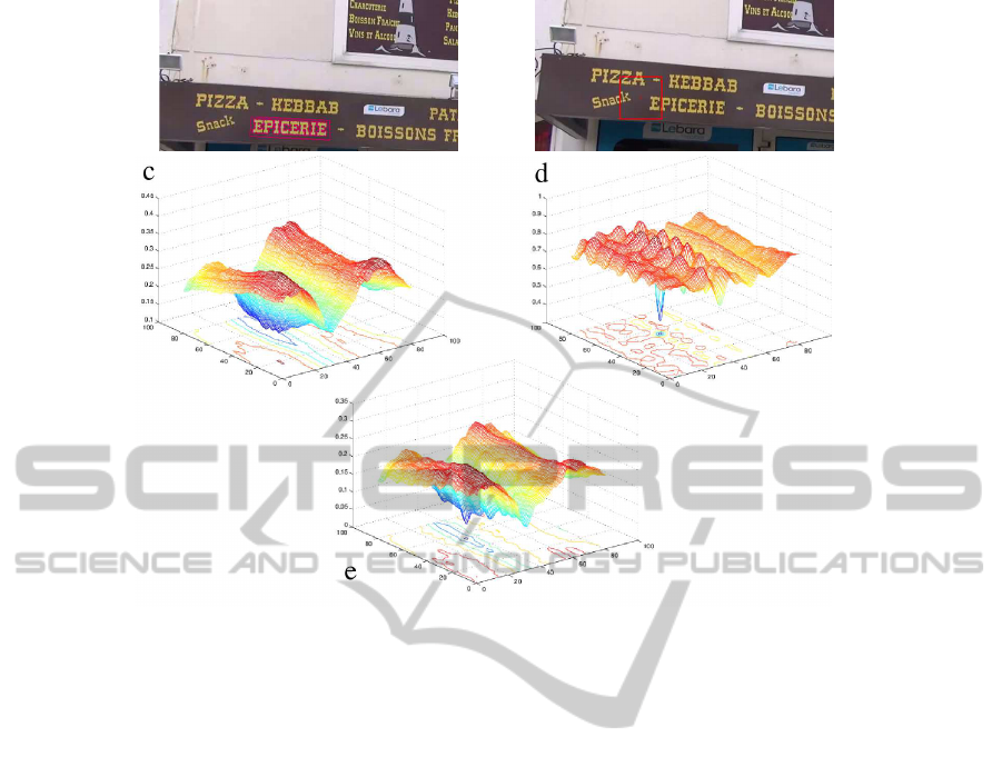
(a) (b)
Figure 2: Distance surfaces (c-e) computed between each area and the model ((a) magenta) in each pixel of the search space
((b) red). Surfaces are obtained with (c) BD(RHOG), (d) TD and, (c) combination of BD(RHOG) and TD.
3.4 BD and TD Combination
To compare the two previous distances i.e. BD and
TD, we have generated 3D surfaces defined as fol-
lows. A text model was extracted in the first frame of
a sequence (magenta rectangle and contours of seg-
mented letters, Fig. 2.(a)). The search space is defined
in frame 6 as the square of 40× 40 pixels centered on
the previous top left corner estimation of the tracked
text area (red square, Fig. 2.(b)). We have chosen this
example because some text areas are visually simi-
lar to the model in this search space (the text epicerie
to track had similar color and shape to kebbab, pizza
and boissons). The distances are computed in each
pixel of this search space, giving surfaces shown in
Fig. 2.(c-e). These distance surfaces should have a
global minimum around the solution (close to the top
left corner location of the tracked text area) and a
slope to reach it. In such cases, w
(i)
t
= e
−αd
2
should
have high values.
Fig. 2.(c) shows the surface given by BD between
RHOGs: (BD(RHOG)). We can see that further par-
ticles have a high distance but this surface has no
peaked global minimum but rather presents a valley
along the text direction (horizontal). Then, all parti-
cles located in this latter have a high weight, even if
they are far from the solution. PF will provide an es-
timation in any point along the bottom of this valley.
That is not satisfactory because too much imprecise.
Fig. 2.(d) shows the surface given by TD between
gray level patches. It presents good properties to pre-
cisely localize the solution into a global minimum.
Unfortunately, the region around this global minimum
is too peaked. As this region is too narrow, only few
particles with high weight will contribute to the esti-
mation (weighted sum) of the tracked text. Elsewhere
TD gives approximately the same high values which
means that particles’ weights are low and irrelevant.
As (BD(RHOG)), TD seems not to be reliable be-
cause, integrated into PF, it requires that at least a few
particles are drawn near the solution. If not, PF will
diverge and then fail.
To take advantage of both presented configura-
tions, we propose to combine (multiply) BD(RHOG)
and TD. The usage of this combination (noted
BD(RHOG)×TD) in a particle filter gives a robust
text tracker. It is our selected solution called TextTrail.
The result of the combination is shown in Fig. 2.(e).
This surface has both the property of BD(RHOG) to
converge to the solution (valley), and the precision of
its localization (peak of TD surface). Thus, particles’
weights will be computed so that w
(i)
t
= e
−α(d
bd
×d
td
)
2
.
TextTrail-ARobustTextTrackingAlgorithmInWildEnvironments
271
4 EXPERIMENTAL RESULTS
In this section, we evaluate TextTrail, our text track-
ing algorithm. First, we compare several likelihood
functions used in the framework of the PF: common
ones and new ones we build. We especially focus
on the impact of the TD on tracking performances to
validate the likelihood function we have introduced.
We have created a batch of video to prove the robust-
ness of our method. Secondly, we intended to com-
pare TextTrail with other algorithms but unfortunately
only a few are dedicated to text tracking and none
provides source codes. Nevertheless, performances
of Snoopertrack (Minetto et al., 2011) are given, and
datasets are online available, so we can compare our
method with their. Finally, to illustrate an interest of
our method, we integrate our text tracker into a com-
plete framework dedicated to online text removing in
video sequences.
4.1 Likelihood Evaluation
4.1.1 Our Challenging Dataset
To test the robustness of several likelihood functions,
the dataset must be as challenging as possible. Our
dataset contains seven 1280 × 720 pixel video se-
quences, captured in wild environment i.e. under un-
constrained conditions in natural scenes (indoor and
outdoor environments). These video and their associ-
ated ground truth (GT) are in the same XML format
as in ICDAR (ICDAR, 2013) and publicly available
1
.
Note that texts in those video are affected by many
and varied difficulties such as: translations, rotations,
noise, stretching, changing in point of view, partial
occlusions, cluttered backgrounds, motion blur, low
contrast, etc. Moreover, same texts can be close to
each others and share visual similarities, thus perturb
trackers. Fig. 4 shows some frame examples for each
video used in our experiment part.
4.1.2 Comparison of Configurations
We compare the efficiency of 5 trackers relying on
different configurations: BD(HOG), BD(RHOG),
TD, BD(HOG)×TD and BD(RHOG)×TD). For all
of them, the model(s) is(are) initialized in the first
frame from their corresponding GT, then tracked
during 100 to 200 frames without any update of
model(s). To evaluate and compare the different con-
figurations, we compute the Fscore which combines
precision and recall, given by:
1
https://www.lrde.epita.fr/∼myriam
Precision =
Overlap
Sur f ace
Track
Recall =
Overlap
Sur f ace
GT
Fscore =
2×(Precision×Recall)
Precision+Recall
This measure depends on the spatial overlap between
the non-rectangular areas of GT and prediction from
the tracker. Sur f ace
Track
is the number of pixels in
the predicted region and Sur face
GT
is the number of
pixels in the GT. Overlap is the number of pixels in
both previous surfaces. Note that, because no one
of our proposed configurations handles size change
while GT does, it is impossible to reach a Fscore of
100% even if, visually the tracking seems to be cor-
rect. Due to the stochastic nature of PF, each tracker’s
Fscore is an average over 50 runs. Note that the cor-
rection parameter α used for weight computation has
a strong influence on the performance of the tracker:
it reshapes the profile of the likelihood (Lichtenauer
et al., 2004) (Fontmarty et al., 2009) (Brasnett and
Mihaylova, 2007). Therefore, for a fair comparison
between each configuration, we tuned its α so that it
yields best tracking results.
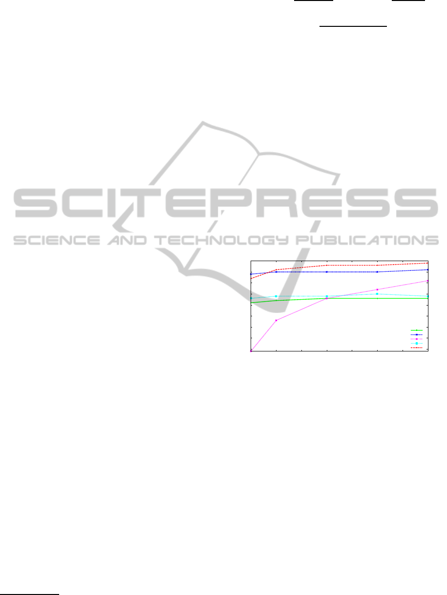
40
45
50
55
60
65
70
75
80
50 100 150 200 250 300 350 400
Fscore (%)
Number of particles
BD(HOG)
BD(RHOG)
TD
BD(HOG)xTD
BD(RHOG)xTD
Figure 3: Convergence curves.
4.1.3 Likelihood Selection
Fig. 3 shows evolutions of Fscore values (aver-
age over 50 runs for each tracked text areas in
all test sequences) when number of particles N in-
creases. One can note that TD needs a lot of
particles to achieve a high Fscore. BD(HOG),
BD(RHOG) and BD(HOG)×TD are more stable
since they quickly converge. Best Fscores are pro-
vided by BD(RHOG)×TD (red curve) from N = 100
and are still slowly increasing with N. As most Fs-
cores are stabilized from N = 200, we have chosen to
perform our tests with this number of particles.
Table 1 presents Fscores (average over 50 runs
for each tracked text areas in all test sequences) with
N = 200. For each Fscore, the standard deviation over
the 50 runs is given in square bracket.
We can observe that TD often gives best Fscore
results, combined with BD(RHOG) or not. Because
VISAPP2015-InternationalConferenceonComputerVisionTheoryandApplications
272

Table 1: Fscores for all trackers with their optimal α value and N = 200. Max Fscores per text are represented in bold and
max average Fscores and min standard deviations in red.
Tracked texts
BD(HOG)
BD(RHOG)
TD
BD(HOG)×TD
BD(RHOG)×TD
# Frames
Fig.3.1. LAVERIE 76.49 [0.60] 89.98 [1.70] 96.45 [0.36] 77.51 [1.02] 95.00 [0.84] 71
Fig.3.1. LIBRE 59.64 [1.88] 77.12 [1.06] 79.02 [7.71] 67.77 [7.08] 84.16 [7.61] 71
Fig.3.1. SERVICE 46.42 [2.34] 46.02 [10.29] 52.34 [13.27] 46.24 [2.65] 47.90 [9.2] 71
Fig.3.1. WASH 58.85 [1.22] 64.61 [1.36] 73.08 [8.14] 64.92 [2.84] 74.50 [3.90] 71
Fig.3.1. SERVICE 31,31 [2.07] 44,93 [7.88] 53,44 [4.81] 32,88 [1.79] 51,74 [10.59] 71
Fig.3.2. DEFENSE 82.69 [0.90] 86.35 [1.39] 72.73 [12.29] 82.73 [0.91] 87,55 [4.75] 207
Fig.3.2. FUMER 37.61 [8.46] 78.24 [4.68] 48.51 [28.09] 53.97 [5.21] 84.61 [6.71] 207
Fig.3.3. THERMOS 58.10 [2.76] 78.29 [0.11] 87.59 [0.04] 62.04 [4.57] 78.15 [0.34] 134
Fig.3.4. RESTAURANT 83.40 [0.62] 88.93 [0.20] 47.46 [3.98] 61.10 [15.46] 81.75 [0.54] 201
Fig.3.5. CONTROL 75.83 [0.25] 78.76 [0.40] 83.32 [0.19] 78.11 [0.44] 83.47 [0.11] 131
Fig.3.6. VOYAGE 86.50 [0.81] 95.34 [1.38] 9.37 [7.97] 84.04 [0.56] 92.44 [1.50] 159
Mean 63.35 75.32 63.94 64.66 78.30
Std 19.18 16.90 24.72 15.94 15.24
of the too much peaked global minimum of TD (see
Section 3), its results are not stable: Fscores can be
either high (Laverie) or low (Voyage). Its standard
deviation is higher than other ones. Therefore, the
unreliability of TD makes it unusable alone. When
it low-performs, its combination with BD(RHOG) al-
lows to reach an higher Fscore (see for example the
case of words Fumer or Voyage).
Notice also, that the RHOG always improves re-
sults compared to HOG (except for Service) when it
is used alone or combined with the TD. This confirms
that the addition of the computation of the HOG on
the boundaries of letters is a powerful improvement.
On words Service, all results are poor. In fact,
the two occurrences of word Service (Fig. 4.1) affect
all trackers because these words are swapped while
tracking. This explains also the high standard devia-
tion of trackers.
Over all tracked texts, our text tracker (called Text-
Trail) with BD(RHOG)×TD combination, gives on
average the higher Fscore (78.3%) on our challenging
video sequences. These experiments have shown that
it is efficient and outperformsa classical approach like
BD(HOG). It takes advantages of both approaches,
the global coarse solution of the BD(RHOG) and the
local and precise solution of the TD.
4.2 Comparison with Another
Approach
Here, we compare our TextTrail with Snooper-
Track (Minetto et al., 2011) in terms of scores and
computation times. Algorithm SnooperTrack re-
lies on detection steps processed every 20 frames:
model(s) of their tracked text(s) are then regularly up-
dated. On the contrary, our method only initializes
models by detecting text areas in the first frame and
keeps the corresponding model(s) constant during the
whole sequence. These approaches are not “fairly
comparable” but SnooperTrack seems to be the most
similar online available algorithm. The comparison is
done on their dataset which is publicly available using
evaluation protocol described in (Lucas, 2005). Note
that our algorithm has been executed on a machine In-
tel i5-3450
c
, 3.1GHz, 8GB of RAM, coded in C++
with our library Olena (Levillain et al., 2010) without
optimization.
Table 2 gives for each video of the dataset, recalls,
precisions, Fscores and average processing times per
frame obtained by TextTrail and SnooperTrack.
One can see that in average on these 5 sequences,
TextTrail reaches the higher Fscore (0.67) and the
higher precision (0.74) rates. Moreover, it is on aver-
age more than two times faster (0.21 sec. per frame)
than the other method (0.44 sec. per frame). Note
that we do not know if computation times of Snoop-
erTrack also include detection times or just tracking.
Apart for the video “Cambronne”, our average com-
putation times are 5.5 times faster (0.0775 sec. per
frame). Note that “Cambronne” sequence is partic-
ular as it contains many text areas localized on the
frame borders: models, restricted to the visible part
of the particle, have to be recomputed. We have not
optimized this part of our algorithm, which explains
the higher computation times obtained for this video.
Our precision rates are always higher (0.74 vs.
TextTrail-ARobustTextTrackingAlgorithmInWildEnvironments
273
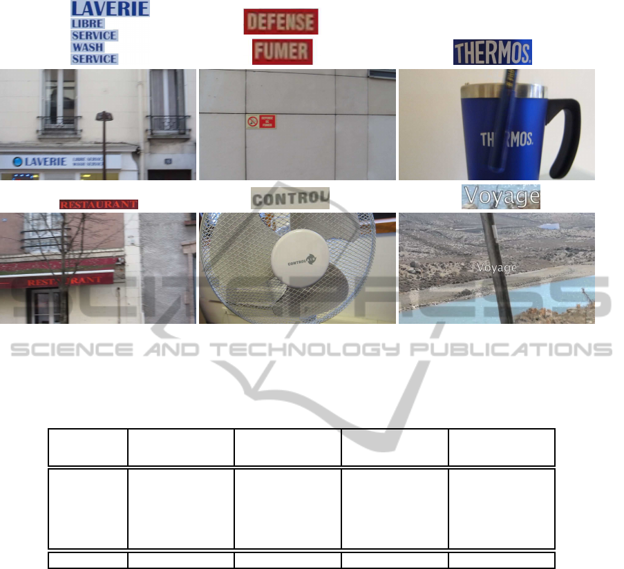
1 2 3
4 5 6
Figure 4: Our challenging video sequences. 1-2: motion blur, 3-4: partial occlusion, 5: rotation, 6: cluttered background.
Zoom on text models to track (extracting from the first frame) are given above each frame.
Table 2: Comparison of performances and execution times between our tracker
TextTrail and the tracker with detection (every
20 frames)
SnooperTrack. Max recall, precision and Fscores per video in bold and minimum average computation times (in
seconds) per frame in bold.
Recall Precision Fscore T(s)
Video
SnooperTrack TextTrail SnooperTrack TextTrail SnooperTrack TextTrail SnooperTrack TextTrail
v01-Bateau 0.80 0.80 0.55 0.80 0.63 0.80 0.19 0.03
v02-Bistro 0.74 0.67 0.57 0.77 0.64 0.72 0.45 0.15
v03-Cambronne 0.53 0.51 0.60 0.67 0.56 0.58 0.88 0.73
v04-Navette 0.70 0.39 0.73 0.74 0.71 0.51 0.15 0.05
v05-Zara 0.70 0.71 0.60 0.73 0.63 0.72 0.55 0.08
Mean 0.69 0.62 0.61 0.74 0.63 0.67 0.44 0.21
0.61). This shows our prediction areas most of times
is included in the GT. However, our recall rate is lower
(0.62 vs. 0.69). As our model size is fixed over time,
even if TD handle small size changes, our predicted
text area size does not change. This is why our recall
rates are smaller. Our predictions of text areas are
then well localized but the scale is not well adapted to
the GT to get higher recall rates.
Furthermore, “v04-Navette” sequence shows an
explicit example of limitation of our approach. In
this video, text area sizes are hardly changing with
time. Our algorithm succeeds to track text up the TD
reaches its limits i.e. when it can not manage high
scale changes. This is why we added a simple cri-
terion (based on the difference of prediction scores
in successive frames i.e. weight(s) of predicted text
area(s)) to stop our tracker(s) in such cases.
Thanks to the TD, robust to small transformations,
this is not necessary to include the corresponding
transformation parameters (scale, for example) into
the state. The state space dimension is then reduced
and we need fewer particles to get an efficient track-
ing.
Without updating the model, TextTrail can track
during hundreds of frames, that prove its robustness.
In practice, to manage apparitions or high changes
in the model (occlusions, illumination, etc.), a detec-
tion step can be launched more often. But, compared
to SnooperTrack, we can track during more than 20
frames without needing to restart tracking from new
detections.
VISAPP2015-InternationalConferenceonComputerVisionTheoryandApplications
274
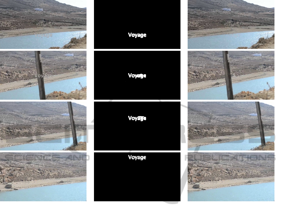
Figure 5: Example of application of our text tracker. First column presents a series of frames (33, 68, 96, 136) with embedded
text. Second column gives binarized text area provided by a tracking and binarization process. Third column shows results of
“inpainted” frames.
4.3 Application: Text Removal
This section is dedicated to an example of applica-
tion of our text tracker. Our goal is to remove text
superimposed on frames of a video sequence. Text-
Trail can locate the text to remove in each frame. This
text is then removed using a classical inpainting algo-
rithm (Bertalmio et al., 2001). In practice, we manu-
ally select a text area in the first frame of the video se-
quence, which is automatically tracked during the se-
quence. A binarization process then provides a mask
which precisely cutouts the text letters. The inpaint-
ing is automatically processed in each frame using
this mask.
Fig. 5 presents different frames of a video from
our dataset: frames with superimposed texts, after the
tracking and binarization process and finally results
of the inpainting procedure. One can see that the text
is correctly localized and then removed. Even if the
result is not “visually perfect”, no one can identify
that something was erased.
5 CONCLUSIONS
In this article, we have presented TextTrail, a new al-
gorithm for multiple text tracking in complex video
sequences relying on a particle filter framework. Even
if the particle filter framework is well known, the
novel idea here, is to combine the Bhattacharyya and
tangent distances in order to increase the efficiency
of the correction step which leads to a more robust
text tracker. According to our experiments, tangent
distance on gray level patches gives a good preci-
sion of the text and Bhattacharyya distance between
“revisited” HOGs adds information on the shape of
letters. High likelihood areas are well localized and
sufficiently smooth for the particle filter to keep a di-
versity of its state representation (i.e. position of the
tracked text area) via the particle set. Unlike clas-
sical approaches from the literature, we show that
our method can track text areas during long times in
video sequences containing complex situations (mo-
tion blur, partial occlusion, etc.) starting from only
TextTrail-ARobustTextTrackingAlgorithmInWildEnvironments
275

one detection step, that is less time consuming. In-
deed, our tracker is initialized by a detection step
and models are never updated, proving the efficiency
of the method. We also show our tracking can be
embedded into a complete framework dedicated to
text removal. If future works, we plan to overcome
the limitation of our approach and allow to manage
stronger transformations. A simple solution is to add
frequent detections to update the model(s). Another
solution is to extend the state space (add scale param-
eters for example). Usually, increasing the state space
means increasing the number of particles to achieve
good tracking performances. But, because tangent
distance can also handle small transformations, state
space should be sampled more coarsely, then using
fewer particles. We think that, even if we increase the
state space dimension, we probably will need fewer
particles to achieve lower tracking errors, and then
also reduce the computation times.
REFERENCES
Bertalmio, M., Bertozzi, A. L., and Sapiro, G. (2001).
Navier-stokes, fluid dynamics, and image and video
inpainting. In CVPR, pages 355–362.
Bhattacharyya, A. (1943). On a measure of divergence
between two statistical populations defined by their
probability distributions. Bulletin of Cal. Math. Soc.,
35(1):99–109.
Brasnett, P. and Mihaylova, L. (2007). Sequential monte
carlo tracking by fusing multiple cues in video se-
quences. Image and Vision Computing, 25(8):1217–
1227.
Breitenstein, M. D., Reichlin, F., Leibe, B., Koller-Meier,
E., and Gool, L. V. (2009). Robust tracking-by-
detection using a detector confidence particle filter. In
ICCV, pages 1515–1522.
Dalal, N. and Triggs, B. (2005). Histograms of oriented
gradients for human detection. In CVPR, pages 886–
893.
Fabrizio, J., Dubuisson, S., and B´er´eziat, D. (2012). Motion
compensation based on tangent distance prediction for
video compression. Signal Processing: Image Com-
munication, 27(2):153–171.
Fabrizio, J., Marcotegui, B., and M.Cord (2013). Text de-
tection in street level image. Pattern Analysis and Ap-
plications, 16(4):519–533.
Fontmarty, M., Lerasle, F., and Danes, P. (2009). Likelihood
tuning for particle filter in visual tracking. In ICIP,
pages 4101–4104.
Gordon, N., Salmond, D., and Smith, A. (1993). Novel ap-
proach to nonlinear/non-Gaussian Bayesian state esti-
mation. IEE Proc. of Radar and Signal Processing,
140(2):107–113.
ICDAR (2013). ICDAR 2013 robust reading competition,
challenge 3: text localization in video.
http://dag.
cvc.uab.es/icdar2013competition/?ch=3
.
Levillain, R., Geraud, T., and Najman, L. (2010). Why and
howto design a generic and efficient image processing
framework: The case of the milena library. In ICIP,
pages 1941–1944.
Lichtenauer, J., Reinders, M., and Hendriks, E. (2004). In-
fluence of the observation likelihood function on ob-
ject tracking performance in particle filtering. In FG,
pages 227–233.
Lucas, S. M. (2005). Text locating competition results. In
Proceedings of the Eighth International Conference
on Document Analysis and Recognition, ICDAR ’05,
pages 80–85.
Macherey, W., Keysers, D., Dahmen, J., and Ney, H.(2001).
Improving automatic speech recognition using tangent
distance. In ECSCT, volume III, pages 1825–1828.
Mariani, R. (2002). A face location and recognition sys-
tem based on tangent distance. In Multimodal inter-
face for human-machine communication, pages 3–31.
World Scientific Publishing Co., Inc.
Medeiros, H., Holgun, G., Shin, P. J., and Park, J. (2010).
A parallel histogram-based particle filter for object
tracking on simd-based smart cameras. Computer Vi-
sion and Image Understanding, (11):1264–1272.
Merino, C. and Mirmehdi, M. (2007). A framework towards
real-time detection and tracking of text. In CBDAR,
pages 10–17.
Minetto, R., Thome, N., Cord, M., Leite, N. J., and Stolfi, J.
(2011). Snoopertrack: Text detection and tracking for
outdoor videos. In ICIP, pages 505–508.
Phan, T. Q., Shivakumara, P., Lu, T., and Tan, C. L. (2013).
Recognition of video text through temporal integra-
tion. In ICDAR, pages 589–593.
Schwenk, H. and Milgram, M. (1996). Constraint tangent
distance for on-line character recognition. In ICPR,
pages 515–519.
Simard, P., LeCun, Y., Denker, J., and Victorri, B. (1992).
An efficient algorithm for learning invariances in
adaptive classifiers. In ICPR, pages 651–655.
Tanaka, M. and Goto, H. (2008). Text-tracking wearable
camera system for visually-impaired people. In ICPR,
pages 1–4.
Tuong, N. X., M¨uller, T., and Knoll, A. (2011). Robust
pedestrian detection and tracking from a moving vehi-
cle. In Proceedings of the SPIE, volume 7878, pages
1–13.
VISAPP2015-InternationalConferenceonComputerVisionTheoryandApplications
276
