
A Linear Physical Programming Approach to Power Flow and
Energy Storage Optimization in Smart Grids Models
Gabriella Dellino
1
, Carlo Meloni
1,2
and Saverio Mascolo
2
1
Istituto per le Applicazioni del Calcolo (IAC) – CNR, Bari, Italy
2
Politecnico di Bari, Bari, Italy
Keywords: Optimal Power Flow, Energy Storage, Smart Grids, Planning, Optimization, Uncertainties.
Abstract: The Optimal Power Flow problem (OPF) plays a crucial role in the successful energy management of
modern smart grids. The diffusion of renewable energy sources poses new challenges to the power grid in
which integrated energy storage combined with green generation solutions can help to address challenges
associated with both power supply and demand variability. This work refers to a smart grid context and
proposes a time indexed OPF model considering storage dynamics, adopting a preference-based
optimization method with chance constraints to provide a suitable service level.
1 INTRODUCTION
Optimal Power Flow problem (OPF) plays a crucial
role in the successful management of modern power
grids.
The diffusion of renewable energy sources (even
in the demand side) poses new challenges to the
power grid in which integrated energy storage
combined with green generation solutions can help
to address challenges associated with both power
supply and demand variability (Chandy et al., 2010,
Koutsopoulos et al., 2011).
This paper reports on some optimization
modeling results of a research work which refers to a
smart grid context and proposes a time indexed
Optimal Power Flow (OPF) model which considers
storage dynamics and adopts a preference-based
optimization method (on the generation side) joined
with a chance constrained approach (on the demand
side) to provide a suitable level of service.
2 PROBLEM DESCRIPTION
The OPF is a class of constrained optimization
problems over a set of power/flow network variables
(Carpentier, 1962). In general the variables may
include active and reactive power outputs, generator
or bus voltages and phases; while the objective may
be the minimization of generation costs or the
maximization of user utilities or level of service; and
the constraints may be bounds on voltages or power
levels, or that the line loading not exceeding thermal
or stability limits. The OPF has been deeply studied
during the last decades and several optimization
techniques have been applied to both model and
solve it (Dommel and Tinney, 1968, Kallrath et al.,
2009).
In this paper, we develop a simple and general OPF
model with energy storage and study how storage
allows optimization of power generation across a
given time horizon considering an uncertain demand
and a system of preferences on the amount of
generated power.
The proposed OPF approach belongs to the family
of energy planning models (Huang et al., 2012,
Khalid and Savkin, 2010) and aims to find a one-
day-ahead energy production and distribution plan
determining:
a) how much load (i.e. demand) to satisfy;
b) when and how much power to draw from the grid;
c) when and how to charge the energy storage
system;
d) how to sell power back to the grid; while the goal
is to minimize the overall costs including energy,
devices and operations.
Besides OPF, which aims to search for the
conditions which give the lowest cost for energy
generation, storage and delivery, the implementation
of the planning results may be based on different
224
Dellino G., Meloni C. and Mascolo S..
A Linear Physical Programming Approach to Power Flow and Energy Storage Optimization in Smart Grids Models.
DOI: 10.5220/0005293602240231
In Proceedings of the International Conference on Operations Research and Enterprise Systems (ICORES-2015), pages 224-231
ISBN: 978-989-758-075-8
Copyright
c
2015 SCITEPRESS (Science and Technology Publications, Lda.)
actuation strategies including Demand Shaping
(DS) and Energy Storage (ES).
The first is based on the (tentative) consumer
demand shaping through financial incentives;
encourages the consumer to: use less energy during
peak hours and/or shift the time of energy use to off-
peak times (i.e. night time, weekends). In the
approach based on Energy storage (ES) ad-hoc units
are required to store energy during off-peak hours
and to discharge (i.e., supply energy) during peak
hours (power leveling).
3 OPTIMAL POWER FLOW
INCREMENTAL MODELING
Developing the Optimal Power Flow model we
adopt an incremental approach interactively
involving decision-makers (e.g., as suggested by
Sierhuis and Selvin (1996)).
We start from a Conceptual Model (proposed by
Chandy et al., 2010) as the basis to develop more
complex and detailed models according to the needs
and the practice of the context.
3.1 Conceptual Model
The Conceptual Model refers to a Single-Bus and
Single-Generator case, but it can be extended to a
network, i.e., Multi-Bus and Multi-Generator cases.
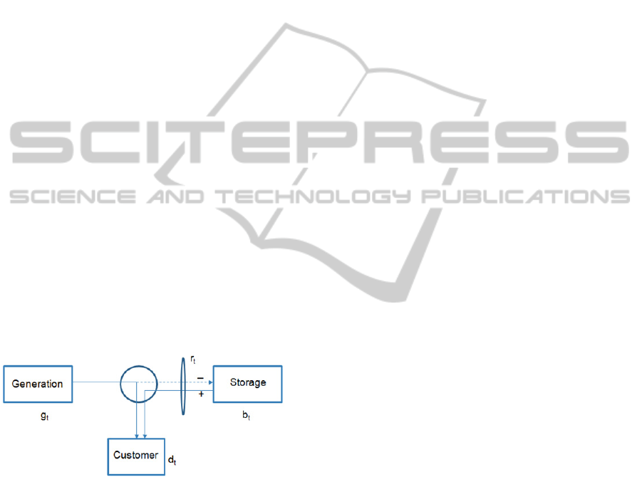
Figure 1: Reference scheme for the Conceptual Model
with respect to a single node
i
of the grid.
The OPF Conceptual Model refers to the scheme
depicted in Figure 1. It is a simple and general OPF
model with energy storage and time-varying
generation costs and power demand. It considers a
single generator connected to a single load; the so
called electric “per unit” DC model is assumed
leading to a simplified structure of the network in
which no reactive power is considered (Chandy et
al., 2010). The main difference from the classical
OPF is that storage allows optimization across time,
e.g. charge when the cost of generation is low and
discharge when it is high.
For each node i of the grid, the considered
Conceptual Model is a time-indexed optimization
problem characterized by a planning horizon
containing
T
time slots
t
(i.e.
t1,…,T
) of the same
length.
For each time slot t is known a value
d
t
for the
power demand. The variables of the problem are the
power
g
t
to be generate in time slot
t
, and the level
of charge
b
t
of the storage system in the time slot
t
,
which has a limited capacity of
B
. The energy flow
to and from the storage system is indicated as
r
t
, i.e.,
assuming positive values while batteries are
supplying energy and negative otherwise.
The considered optimization model includes a first
set of demand satisfaction constraints, and set of
constraints dealing with the level of charge of the
batteries, while all variables are required to be non-
negative.
The objective function is a cost to be minimized
containing a generation and a storage component.
The generation cost
can be assumed to be
quadratic and (possibly) time-varying. The
convexity of the cost function reflects a possible
decreased efficiency when producing very high
amounts of power (Chandy et al. 2010).
The storage cost
hb
t
is assumed to be dependent
only on the state of charge
b
t
(and not on the charge
or discharge rate); it can be formulated as a linear
penalty term for deviation from the desired target.
An additional component
kb
T
could be included to
represent an optional penalty for the deviation from
a final target value
b
T
(i.e.,
b
t
with
tT
) of the state
of charge.
The overall formulation leads to the following
mathematical program:
∑
(1)
subject to (for all t = 1,…, T):
(2)
(3)
0
(4)
0
(5)
0(6)
3.2 Case Study: Problem Setting and
Preliminary Results
We consider, as “basic” case study, a problem
introduced by Chandy et al. (2010) to illustrate the
characteristics of the Conceptual Model reported in
Section 3.1. This problem refers to a single-bus and
ALinearPhysicalProgrammingApproachtoPowerFlowandEnergyStorageOptimizationinSmartGridsModels
225
single-generator case under the assumption of an
electrical “per unit” DC model.
The considered planning horizon is
T24
hours
and each time step
t
has a duration of
1
hour.
According to the original model, the demand (in GJ
units) profile in the planning horizon is represented
by:
5010sin
(7)
The energy storage system is characterized by a
battery capacity
B25
GJ, and an initial level of
charge
b
0
12.5
GJ.
The additive components to the cost function
Z
−to
be minimized− are:
0.5
(8)
(9)
As proposed by Chandy et al. (2010), in our “basic”
case study some simplifications are included: i) the
last component, related to the final level of charge of
the batteries, is obmitted; ii) the cost coefficient is
constant in the planning horizon and fixed to
γ
t
1
for all
t
(invariant case) While the value of the
coefficient a was set to
2
.
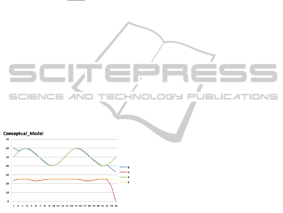
Figure 2: Conceptual Model Results for the basic case
study. The
x
-axis reports the time slots,
y
-axis indicates
power levels.
As depicted in Figure 2, according to Chandy et al.
(2010), the optimal generation
g
t
is linear when the
batteries charge and discharge, and follows the
demand when the storage system is at the maximum
level of charge. In the particular illustrative problem
setting, the storage system is hardly used at all and
appears quite oversized. In fact, it is mainly due to
the relative values of generation and storage costs
and their invariance in the planning horizon.
The energy storage system clearly needs a better
modeling to deal with the level of charge at the end
of the period. The decision-makers needs to consider
in the planning activities also the preference and
limitations on the generation-side and the possible
uncertainties on the demand-side.
3.3 OPF: Enhanced Models
Starting from the Conceptual Model, and on the
basis of the requirements defined in the application
context, we are working, together with the decision-
makers, on several modeling extensions mainly
devoted to address the following issues, which
compose our current research agenda:
1. Limitations on the flows to/from the storage
system in each time slot;
2. Generated flow possibly assumes negative values
(i.e., the Distribution System Operator (DSO)
should receive energy from the node);
3. Demand predictions possibly assume negative
values (i.e., customers should produce energy);
4. (Upper/Lower) Bounds on the amount of
generated energy (possibly negative), e.g.,
a) constant bounds;
b) time-dependent (yet known) bounds;
c) preferences (penalty based) on the level of
power generation;
5. Uncertainties affecting the demand forecasts
d
t
;
6. Storage system inefficiencies with respect to
holding, discharging and recharging phases;
7. Possible different energy sources;
8. More specific constraints related to the discharge
and recharge phases of specific classes of energy
storage systems;
9. Extension to a multi-generator and multi-bus
context.
In particular, in this work we address the modeling
issues related to points 4 and 5.
3.3.1 Uncertain Demand Forecasts
In general, uncertainties affecting the demand
forecasts
d
t
are described as prediction intervals and
error distributions (Box et al., 2008, Pflug and
Römisch, 2007, Narayanaswamy et al., 2012,
Conejo et al., 2010). On the basis of a demand
forecast, the planner receives, for each time slot, the
predicted value (i.e.,
d
t
), the prediction interval, and
the distribution of the values inside that interval.
On the basis of the forecasting values distribution
within the prediction interval (e.g., from
Autoregressive Integrated Moving Average
ICORES2015-InternationalConferenceonOperationsResearchandEnterpriseSystems
226
(ARIMA) or Support Vector Machines (SVM) time
series models) we adopt a chance constrained
approach (Charnes and Cooper, 1959) introducing a
new set of constraints −to replace constraints (2) in
the Conceptual Model (1)-(6)− in order to guarantee
a given probability of demand satisfaction:
Prg
t
r
t
d
t
1‐αfort1,...,T
(10)
They represent a set of Level-of-Service (LOS)
constraints and –noting that the uncertainty affects
only the r.h.s of each constraint– can be linearized
(Vanderbei, 2001) using the critical value
d
’
t
associated to
α
(i.e., the specific required level of
probability) through the probability density function
of the demand:
g
t
r
t
d'
t
fort1,...,T
(11)
Using these set of constraints instead of (2) leads to
a first enhanced model, hereinafter indicated as
EM1.
3.3.2 EM1: Additional Problem Settings and
Results
To test the enhanced model EM1, the basic case
study has been modified to consider the demand
uncertainties. The forecasted demand value (i.e., the
expected value) is assumed to be given by equation
(7) for each time slot
t
.
The effect of prediction uncertainties has been
modelled as a demand characterized in each time
slot by a normal distribution (other distributions can
be used instead) with mean given by the expected
value
d
t
(i.e., through equation (7)). Two different
scenarios has been considered. The first is
characterized, in each time slot, by a standard
deviation
σ
5%
0.05d
t
, while the second by
σ
10%
0.1d
t
. The probability of demand satisfaction
is set to obtain 3 scenarios for the level of service
(LOS):
70%
;
80%
and
90%
, respectively
(according to equation (10)).
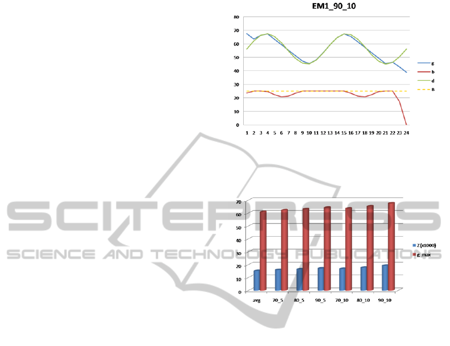
As an example, Figure 3 reports the results obtained
by EM1 in the scenario characterized by a LOS of
90%
and the higher demand variability.
Due to more severe demand requirements, the use of
the storage system increases in the optimal plan. The
optimal generation
g
t
holds an almost linear
behavior when the storage charges and discharges,
and still matches the demand when the storage
system is saturated. The storage system still calls
for a better consideration of the behavior at end of
the period.
Figure 3: EM1 Results for the case study with
LOS90%
and σ
10%
.
The
x
-axis reports the time slots,
y
-axis indicates
power levels.
Figure 4: EM1 results for all scenarios: costs
Z
and the
maximum generated power
g_max
.
Decision-makers acknowledge the practical
relevance of this approach on the demand-side but
they need to improve the model on the generation-
side to allow a better management of the amount of
generated energy.
More specifically, decision-makers find this models
not comfortable as the
g_max
is close (or even over)
the generation capacity of the node, and they are
called to negotiate additional power to/from other
nodes of the grid.
Figure 4 shows the results for all the scenarios in
terms of the total cost
Z
and the maximum generated
power
g_max
in the time slots within the planning
period. In this figure, the scenario indicated as “avg”
represents the base original scenario in which the
expected values of the demand
d
t
are considered for
each time slot (i.e., without demand variability).
Other different scenarios are indicated in the x-axis
with a label XX_Y, where XX represents the
required LOS, and Y the amount of demand
variability (i.e.,
σ
5%
or
σ
10%
).
ALinearPhysicalProgrammingApproachtoPowerFlowandEnergyStorageOptimizationinSmartGridsModels
227
3.3.3 A Preference-based Generation
Management
In their planning activity, decision makers are
subject to limitations in the amount of power that
can be generated. Clearly, this issue can be easily
addressed introducing a direct (and constant) bound
on all the
g
t
variables.
More in general, we can consider the case with time-
dependent (yet known) bounds in which, for each
node of the grid, we introduce a capacity
G
t
MAX
that
bounds the value of
g
t
. Nevertheless, decision
makers are used to reason in terms of operative
ranges, an approach which is only partially
supported by a quadratic model for the generation
costs as considered in the conceptual model and in
EM1.
The need expressed by decision makers suggest us
to setup a new enhanced model EM2 including the
generation management with preferences on the
different possible operative ranges.
In this modeling extension, these preferences are
taken into account by a (linear) progressive penalty
system.
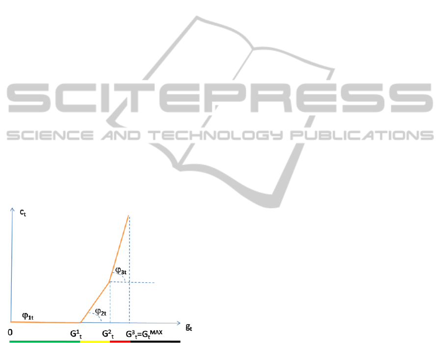
The operative ranges in the feasible range
0,G
t
MAX
indicated by the decision makers are represented in
Figure 5 and are characterized as follows:
Figure 5: the generation cost
c
t
with a progressive linear
penalty system based on different operative ranges.
OPERATIVE_RANGE 1 (OR1):
0, G
1
t
this
operational region is “preferred” or
“desirable” and has an associated NULL
penalty (in Figure 5 it is indicated in green)
assuming
φ
1
t
0;
OPERATIVE_RANGE 2 (OR2):
G
1
t
, G
2
t
this
region is considered “tolerable” (indicated in
yellow in Figure 5), and has a penalty
described by a slope
φ
2
t
0;
OPERATIVE_RANGE 3 (OR3):
G
2
t
, G
3
t
these
values are “undesirable” (yet feasible, they
are marked in red in Figure 5) and have a
penalty represented by the slope
φ
3
t
, with
φ
3
t
0.
The level
G
3
t
coincides with
G
t
MAX
which indicates
the production capacity of the system, i.e., any
generation level
g
t
G
t
MAX
is not feasible (in Figure
5 it is indicated in black).
For any feasible value
g
t
of energy generated in the
time slot
t
, the cost is composed by a base-cost
given by c
t
g
t
and the additional penalty components
depending on the region belonging
g
t
.
The system of penalties is formulated introducing a
new set of constraints in the OPF model.
The first group of constraints takes into account the
generation capacity in each time slot:
1,…, (12)
For each
ORi
and for each time slot
t
, we introduce a
new set of variables
it
0
representing the
displacement in that operative range of the power
generated during the time slot
t
. These displacement
variables are required to satisfy, for each operative
region
ORi
with
i2
, the following constraints:
1,…, (13)
The additional (linear) contribute to the cost function
for each time slot
t
is given by:
∑
(14)
with
,
, and
0.
All these elements, in addition to the extensions
already considered in EM1 lead to a new enhanced
model we indicate hereinafter as EM2.
The weights
W
it
(and so slopes
φ
it
) are determined
on the basis of additional indications provided by the
decision makers.
More specifically, as the range limits define the
preference internally to each single time slot (i.e.,
intra-period), they suggest a particular One-Versus-
Other (OVO) rule to describe their inter-period
preferences.
In fact, they prefer to minimize “as a priority” the
number of “red” time-slots (i.e., those showing a
positive displacement in
OR3
) and the amount of
energy belonging in that region, and then those in
“yellow” (i.e., the time slots limiting the power
generation, at most, to
OR2
).
Overall, the preference based system
proposed/shared with the decision makers belongs to
ICORES2015-InternationalConferenceonOperationsResearchandEnterpriseSystems
228
the family of the so called Linear Physical
Programming (LPP) Models (e.g., see Messac,
1996).
3.3.4 EM2: Additional Problem Setting and
Results
To test the enhanced model EM2, the previous case
study has been enriched. Besides the consideration
of the demand uncertainties, the model of the energy
storage system has been modified considering a
battery capacity
B25
GJ, a battery initial level of
charge
b
0
0.8B
, and the following additional
constraint on the final level of charge:
(15)
and a new set of bounds on the minimum operative
level of charge, required to be at least
b
min
0.05B
:
1,…, (16)
The component of the cost function related to the
energy storage system is the same considered in
EM1, while the base-component of the power
generation cost is linear with a unitary cost given by
c
t
0.5
, considered as constant in all the time slots.
The components of the generation cost, related to the
preference system and the OVO rule, are determined
on the basis of the following
ORi
:
OR1:
0,50,
OR2:
50,57.5,
OR3:
57.5,60,
giving the weights
W
2
0.013
, and
W
3
1
.
The modeling of the demand behavior and its
variability are the same considered in the setting of
the previous case study, as well as the three
LOS
scenarios.
In general, due to the more challenge context, the
use of the energy storage system has increased in all
the considered scenarios playing an important role to
cope with periods characterized by higher demand
levels taking into account the generation constraints.
It is worth to note that the linearity of the generated
power when batteries are charging/discharging does
not hold for EM2. Moreover, the storage system
shows a satisfactory behaviour also in the terminal
phase of the considered planning period.
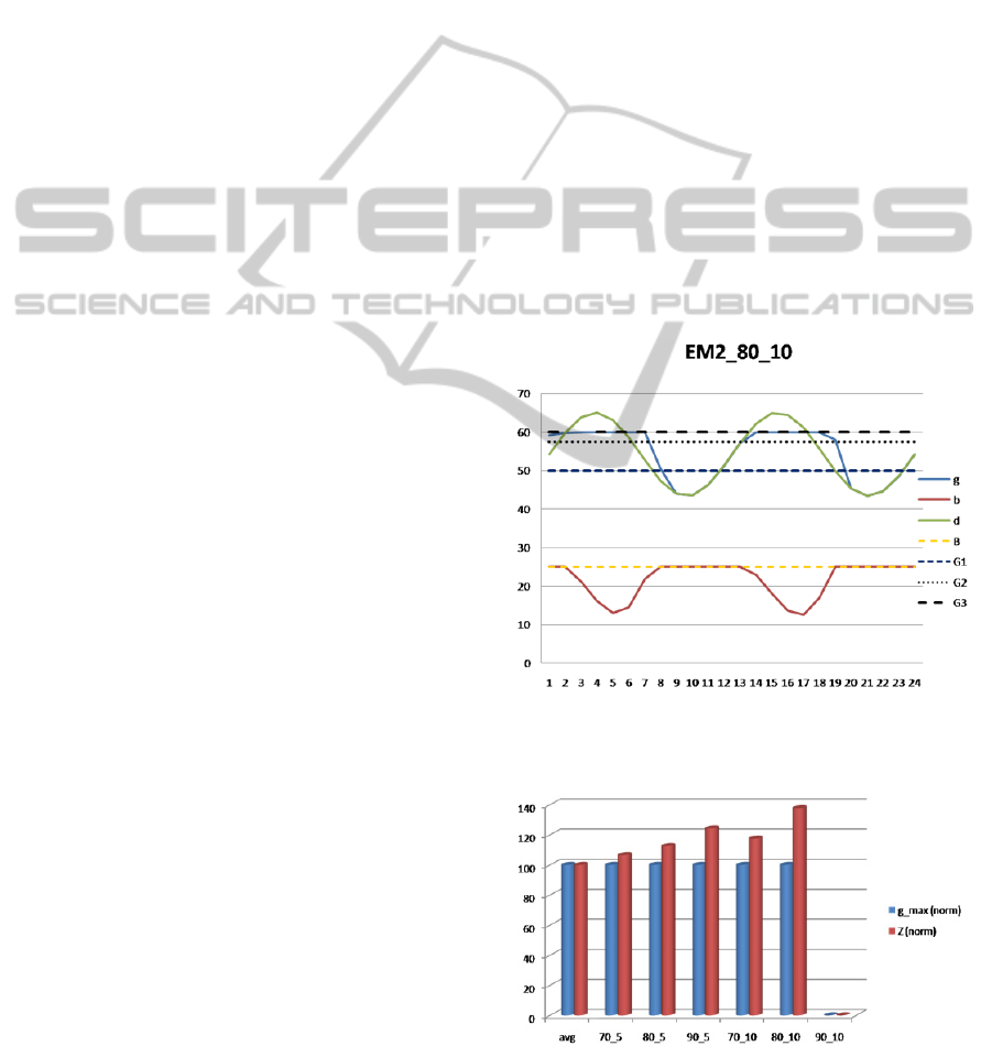
Figure 6 reports a representative sample of the
results obtained by EM2. In particular, the figure
refers to the scenario characterized by a LOS of
80%
and the higher demand variability and clearly shows
the power leveling effect of the energy storage
system which charges during off-peak hours and
discharges during peak hours.
Figure 7 shows the results for all the scenarios in
terms of the total cost Z and the maximum generated
power g_max in the time slots within the planning
period. Again, as in Figure 4, the scenario indicated
as “avg” represents the base original scenario
without the superimposed demand variability, while
other different scenarios are indicated with the same
XX_Y notation. In this case, all the results are
normalized w.r.t. the “avg” scenario and it is clear
how EM2 is able to give an almost constant g_max
among the different scenarios. As expected, these
results show costs increasing as the LOS and the
demand variability increase.
The decision makers, on the basis of the results
obtained by the enhanced model EM2, often
consider also different corrective actions including
demand shaping (on the demand-side), negotiation
to sell or buy energy (on the grid-side). EM2 gives
useful information to support these management
activities.
Figure 6: EM2 Results for the case study with
LOS80%
and
σ
10%
. The
x
-axis reports the time slots,
y
-axis
indicates power levels.
Figure 7: EM2 results (normalized w.r.t. the “avg”
scenario) for all scenarios: costs
Z
and the maximum
generated power
g_max
.
ALinearPhysicalProgrammingApproachtoPowerFlowandEnergyStorageOptimizationinSmartGridsModels
229
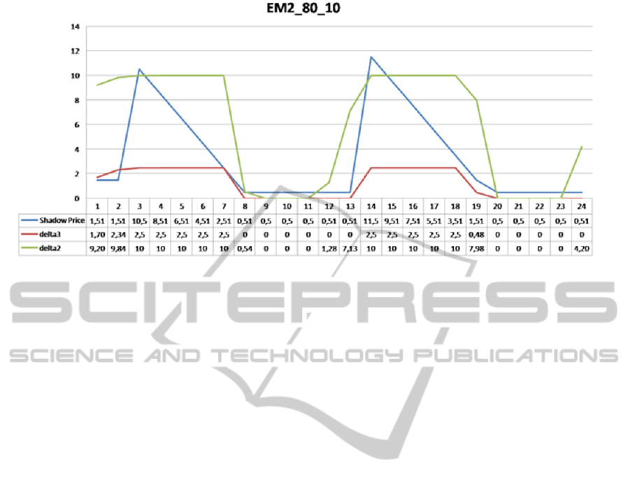
Figure 8: EM2 Results for the case study with LOS = 80% and σ10%. Displacements variables in OR2 and OR3, and
energy shadow prices in each time slot.
Firstly, these information are represented by the
displacement variables in the different operative
regions which indicate the level of production and
its severity in each time slot.
Secondly, this information can be easily
incorporated in a managerial dashboard joined with
an estimation of the marginal value of a power unit
(to sell or buy) in each time slot in the planning
horizon.
EM2 provides this kind of estimation in terms of
shadow prices associated to the demand (
LOS
)
satisfaction constraints. Figure 8 reports −for the
scenario with higher demand variability and a LOS
of
80%
− an example of these useful information in
numerical as well as graphical forms.
4 CONCLUSIONS
In this paper we develop an Optimal Power Flow
model adopting an incremental approach
interactively involving decision-makers.
We start from a simple conceptual model as the
basis to develop more complex and detailed models
according to the needs of the decision-makers trying
to bridging the gap between modeling and the
practice.
The interactive modeling development allows us to
individuate several directions to develop enhanced
models including the extension to networks (i.e.,
Multi-Bus and Multi-Generator cases); the
representation of relevant storage system
inefficiencies and more specific constraints related
to the discharge and recharge phases of specific
classes of energy storage systems.
ACKNOWLEDGEMENTS
This work was supported by the Project "RES
Novae" (Reti, Edifici, Strade - nuovi obiettivi
virtuosi per l'ambiente e l'energia), 2012-2015,
funded by MIUR (Italy).
REFERENCES
Box, G.E.P., Jenkins, G.M., Reinsel G.C., 2008, Time
Series Analysis: Forecasting and Control, 4th ed.
John Wiley & Sons.
Carpentier J., 1962, Contribution to the economic dispatch
problem, Bull. Soc. Franc. Electr.,vol. 3, no. 8, pp.
431-447.
Chandy, K.M., Low, S.H., Topcu U., Xu H., 2010, A
simple optimal power flow model with energy storage,
in Proc. of 49th IEEE Conference on Decision and
Control (CDC 2010), Atlanta, GA, pp. 1051-1057.
Charnes, A., Cooper, W.W., 1959 Chance constrained
programming, Management Science, 6, 73–80.
Conejo A.J., Carrión M., Morales J.M., 2010, Decision
making under uncertainty in electricity markets,
Springer International Series in Operations Research
and Management Science.
Dommel H., Tinney W., 1968, Optimal power flow
solutions, IEEE Transactions on Power Apparatus and
Systems, vol. 87, no. 10, pp. 1866-1876.
Huang, L., Walrand, J., Ramchandran, K., 2012, Optimal
Demand Response with Energy Storage Management,
in Proc. of IEEE Third International Conference on
ICORES2015-InternationalConferenceonOperationsResearchandEnterpriseSystems
230

Smart Grid Communications (SmartGridComm 2012),
Tainan, 61-66.
Kallrath J., Pardalos P.M., Rebennack S., Scheidt, M.,
2009, Optimization in the energy industry,,Springer.
Khalid, M., Savkin, A.V., 2010, Model predictive control
based efficient operation of battery energy storage
system for primary frequency control, in Proc. of 11
th
International Conference on Control Automation
Robotics Vision (ICARCV), 2248–2252.
Koutsopoulos, I., Hatzi, V., Tassiulas, L., 2011, Optimal
Energy Storage Control Policies for the Smart Power
Grid, in Proc. of 2011 IEEE International Conference
on Smart Grid Communications (SmartGridComm
2011), Brussels, pp. 475- 480.
Messac A., 1996, Physical Programming: Effective
Optimization for Computational Design, AIAA
Journal, 34(1). 149-158.
Narayanaswamy, B.; Garg, V.K.; Jayram, T.S., 2012,
Prediction Based Storage Management in the Smart
Grid, in Proc. of 2012 IEEE Third International
Conference on Smart Grid Communications
(SmartGridComm 2012), Tainan, 498-503.
Pflug G.C., Römisch W., 2007, Modeling and managing
risk, World Scientific.
Sierhuis, M., Selvin, A.M., 1996, Towards a Framework
for Collaborative Modeling and Simulation. Proc. of
the Workshop on Strategies for Collaborative
Modeling and Simulation, CSCW'96 Conference,
Boston, USA.
Vanderbei, R.J., 2001, Linear Programming: Foundations
and Extensions, 2nd ed.. Kluwer Academic Publishers,
Dordrecht, Netherlands.
ALinearPhysicalProgrammingApproachtoPowerFlowandEnergyStorageOptimizationinSmartGridsModels
231
