
Weakly Supervised Object Localization with Large Fisher Vectors
Josip Krapac and Sini
ˇ
sa
ˇ
Segvi
´
c
Faculty of Electrical Engineering and Computing, University of Zagreb, Zagreb, Croatia
Keywords:
Weakly Supervised Object Localization, Fisher Vectors, Sparse Classification Models.
Abstract:
We propose a novel method for learning object localization models in a weakly supervised manner, by em-
ploying images annotated with object class labels but not with object locations. Given an image, the learned
model predicts both the presence of the object class in the image and the bounding box that determines the
object location. The main ingredients of our method are a large Fisher vector representation and a sparse
classification model enabling efficient evaluation of patch scores. The method is able to reliably detect very
small objects with some intra-class variation in reasonable time. Experimental validation has been performed
on a public dataset and we report localization performance comparable to strongly supervised approaches.
1 INTRODUCTION
Detecting the presence of objects in images and re-
covering their locations are often jointly addressed
by applying a trained binary classifier at many image
locations, and by reporting objects where a positive
response was obtained. Most successful representa-
tives of this approach (Viola and Jones, 2004; Dalal
and Triggs, 2005; Lampert et al., 2009; Felzenszwalb
et al., 2010; Cinbis et al., 2013) employ strong su-
pervision at the training stage. These methods require
that each training image is annotated with information
about the object location and class. However, annotat-
ing object locations is expensive due to significant hu-
man labeling effort involved, even if a simple location
model is used (e.g. bounding box). This is especially
the case in realistic scenarios when thousands of an-
notations are required to achieve the top performance
(Munder and Gavrila, 2006). Annotation is particu-
larly difficult when the objects of interest are small,
since near to pixel-level annotation accuracy may be
required for best results.
In order to alleviate the effort of full annotation,
several recent papers have tried to solve the object
localization problem in a weakly-supervised manner
(Galleguillos et al., 2008; Siva and Xiang, 2011; De-
selaers et al., 2012; Nguyen et al., 2014; Cinbis et al.,
2014). In this setting, the training images are anno-
tated only with class labels. The training procedure is
supposed to discover the object locations and train the
classifier at the same time. At the test time, however,
bounding boxes have to be predicted for each learned
object class as in the strongly supervised case. This
can be useful even if the recovered object classifier
is not particularly fast, since the recovered localiza-
tion can be used to train a more efficient localization
model in a strongly supervised fashion (Chum and
Zisserman, 2007).
Weakly supervised training of object classifiers
is a daunting task in most realistic scenarios. If
we assume 1000 positive training images and 80000
patches per image, an exhaustive search for object lo-
cations would have to consider 80000
1000
hypothe-
ses. One way to decrease this complexity would be
to avoid checking all patches in positive images by
sampling (Crandall and Huttenlocher, 2006; Crowley
and Zisserman, 2013), clustering (Chum and Zisser-
man, 2007) or employing bottom-up location propos-
als based on trained segmentation (Galleguillos et al.,
2008; Cinbis et al., 2013; Cinbis et al., 2014) or ob-
jectness cues (Siva and Xiang, 2011; Deselaers et al.,
2012). However all these approaches risk to miss
some true object patches at the selection stage, which
may invalidate all subsequent efforts.
A more conservative approach relies on classifiers
able to detect the object presence in a larger image
context. Such classifiers can be trained on positive
images (Nguyen et al., 2014) or image regions (Gal-
leguillos et al., 2008) and then subsequently applied
to recover or gradually improve the object localiza-
tion. Much of the previous work along these lines
(Galleguillos et al., 2008; Nguyen et al., 2014) has
been based on BoW histograms (Sivic and Zisserman,
2003; Csurka et al., 2004) which do not achieve state
44
Krapac J. and Šegvi
´
c S..
Weakly Supervised Object Localization with Large Fisher Vectors.
DOI: 10.5220/0005294900440053
In Proceedings of the 10th International Conference on Computer Vision Theory and Applications (VISAPP-2015), pages 44-53
ISBN: 978-989-758-090-1
Copyright
c
2015 SCITEPRESS (Science and Technology Publications, Lda.)

of the art image classification performance (S
´
anchez
et al., 2013), especially on datasets with small distinc-
tive details (Gosselin et al., 2013). Recently, Cinbis
et al. (Cinbis et al., 2014) have proposed an approach
based on Fisher vector representation which still re-
quires bottom-up location proposals in order to keep
the computations tractable.
In this paper we present a novel weakly-
supervised object localization method based on large
Fisher vectors. The presented method does not re-
quire any bottom-up location proposals and succeeds
to achieve a high localization performance in exper-
iments on very small objects (traffic signs). We ar-
gue that a Fisher vector representation without non-
linear normalizations (power, metric) (S
´
anchez et al.,
2013) is especially well-suited for localizing small
objects (the needle in a haystack scenario (Chum
et al., 2009)) due to its ability to preserve unusual de-
tails (section 3). In order to alleviate computational
complexity caused by a huge dimensionality of large
Fisher vectors, we select a subset of Fisher vector rep-
resentation capable to identify discriminative parts of
the object class by training a sparse linear classifica-
tion model (section 4). The resulting classifier is ap-
plied at all image locations and the spatial layout of
highly scored patches is used to determine the bound-
ing boxes for the detected objects (section 5). This
is similar to the sliding window image traversal, but
much more efficient due to optimizations which take
advantage of the model sparsity (section 6). The pro-
posed method is experimentally validated on a pub-
lic dataset containing very small objects with some
intra-class variation, in front of information-abundant
background as illustrated in Figure 4. We demonstrate
fair localization performance, comparable to strongly
supervised approaches, by evaluating patch scores us-
ing only a fraction (64/1024) of Fisher vector repre-
sentation of the patch (section 7).
2 RELATED WORK
Many previous approaches to weakly supervised lo-
calization adopt the following basic structure: i)
bottom-up initialization of object locations in posi-
tive images, ii) iterative successive improving of clas-
sification and localization models. The second step
typically optimizes a criterion that at least one (Gal-
leguillos et al., 2008; Crowley and Zisserman, 2013)
(or exactly one (Chum and Zisserman, 2007; Siva and
Xiang, 2011; Deselaers et al., 2012; Nguyen et al.,
2014)) object is found in each positive image and that
no objects are found in negative images. This opti-
mization can be viewed as a kind of multiple-instance
learning (Auer, 1997; Andrews et al., 2002) (MIL).
In general, MIL implies training a binary classifier on
bags of instances, such that positive bags contain at
least one positive feature while negative bags contain
all negative features.
Crandall et al. (Crandall and Huttenlocher,
2006) take a random sample of patch descrip-
tors (n=100000) from training images and initial-
izes the training with the most discriminative subset
(n=10000). Several part-based models are then ini-
tialized from descriptor pairs and subsequently op-
timized through EM. Crowley et al. (Crowley and
Zisserman, 2013) search for an initial set of similar
descriptors with one-shot classifiers trained on ran-
dom patches, while further refinement is performed
through MIL. Chum et al. (Chum and Zisserman,
2007) avoid random initialization by starting from vi-
sual words of a BoW representation and proceed in
the MIL fashion. Random initialization can also be
avoided by filtering patch candidates in positive im-
ages. Galleguillos et al. (Galleguillos et al., 2008)
propose to consider regions obtained by multiple
bottom-up segmentations. Each region is represented
as a BoW histogram, and a boosted classifier is con-
structed by repeatedly minimizing the classification
loss in a MIL fashion. Deselaers et al. (Deselaers
et al., 2012) apply a trained generic object detector
(Alexe et al., 2010) to guide initialization of 100 ran-
dom samples in each training image. By assuming
that there is only one object in each positive image
they train a CRF which simultaneously optimizes ob-
ject locations and the classification model. Siva et al.
(Siva and Xiang, 2011) propose a related approach
which focuses on capturing multi-modality of object
appearance. Although some of these approaches are
more advanced than the others, all of them may com-
pletely miss small objects at the initialization step.
Due to that, MIL refinement may easily get trapped
in a local optimum (as confirmed by our preliminary
experiments), and the training is likely to fail. Ad-
ditionally, MIL optimization is computationally very
intensive, so that training on large datasets is not fea-
sible.
Several approaches (Pandey and Lazebnik, 2011;
Nguyen et al., 2014; Cinbis et al., 2014) initialize pos-
itive object locations to entire (or almost entire) pos-
itive images and then attempt to gradually zoom into
correct locations through iteration. One way to for-
mulate this iteration is to represent object locations as
latent variables in a deformable part model framework
(Pandey and Lazebnik, 2011). Another approach
would be to construct an integral image of the patch
scores and to rely on branch-and-bound techniques in
order to find regions which maximize score for the
WeaklySupervisedObjectLocalizationwithLargeFisherVectors
45

current classification model (Nguyen et al., 2014).
Both of these approaches do not require bottom-up
location proposals, however they are prone to conver-
gence issues, while not being able to handle training
images with multiple objects. Finally, this iteration
can also be expressed in terms of bottom-up location
proposals as proposed in (Cinbis et al., 2014). In their
approach, the first classification model is trained on
Fisher vectors of entire positive and negative images.
In each subsequent iteration the negative locations are
chosen as (false) positives of the current classification
model on the negative training dataset. On the other
hand, the positive locations are set to the top-scored
bottom-up location proposals. A care has been taken
to avoid a bias towards the locations from the last it-
eration by performing the training and selection steps
on different folds of the training set of positive im-
ages (this procedure is called multi-fold MIL learn-
ing). This approach currently achieves state-of-the-
art mAP PASCAL visual object classes (VOC) 2007
localization challenge performance of 22.4%.
The method proposed in this paper also harnesses
the Fisher vector representation for weakly super-
vised object localization. However, unlike (Cinbis
et al., 2014), our method identifies the most distinc-
tive parts of the object class by directly applying a
sparse classification model at the patch level
1
. The
main advantage with respect to the majority of other
weakly supervised localization approaches is that we
do not require bottom-up location proposals. Our
method is therefore able to target object classes which
do not receive sufficiently accurate (e.g. 50% IoU)
bottom-up location proposals, which may happen due
to small size or cluttered environment. Additionally,
the capability to be applied at the patch level also en-
tails a potential to achieve high detection performance
(over 80% AP on our dataset).
In comparison with previous approaches (Nguyen
et al., 2014; Chum and Zisserman, 2007) which
also avoid bottom-up proposals, our method is based
on Fisher vectors as a superior image representation
model (S
´
anchez et al., 2013). Thus, our method may
succeed even when the number of BoW components
is not large enough to ensure that distinctive patches
get represented by a dedicated component (cf. Fig-
ure 1). Additionally, we do not use efficient subwin-
dow search (Lampert et al., 2009) to localize win-
dows which maximize overall patch score (Nguyen
et al., 2014), since the background clutter often ob-
structs that approach to the point of producing bound-
ing boxes several times larger than the object. A ma-
1
A similar idea has been explored in (Chen et al., 2013),
however they address a strongly supervised localization and
do not consider sparse classification models.
jor obstacle towards making our method feasible was
to keep the computational complexity tractable with
respect to the dimensionality of image representation
(in our case the Fisher vectors are about 165 times
larger than BoW histograms for the same number of
visual words). We succeeded to achieve that by rein-
forcing a sparse patch classification model.
3 FISHER VECTOR IMAGE
REPRESENTATION
Fisher vectors can be viewed as a way to embed
data points (e.g. patch feature vectors) into a higher-
dimensional vector space. This embedding has a de-
sirable property that the data points which are re-
lated w.r.t. the generative process become close in the
embedded space. Thus one can build advanced dis-
criminative models which achieve improved perfor-
mance thanks to the knowledge of the data distribu-
tion (Jaakkola and Haussler, 1998).
Let the parametric generative model be given with
θ, and let the pdf of a data point x
x
x w.r.t. to generative
model be p(x
x
x|θ). Consider now the score function
(gradient of the log-likelihood) given with:
U(x
x
x|θ) = ∇
θ
log p(x
x
x|θ). (1)
The score U(θ,x
x
x) succinctly describes the relation of
the data point w.r.t. the parameters of the generative
model. Consequently, the data embedded in the score
space may be easier to separate using a linear classi-
fier, since dot product in score space corresponds to
a non-linear kernel in the original space. By decorre-
lating components of the score, we obtain the Fisher
vector Φ(x
x
x|θ) of the data point x
x
x given the generative
model θ:
Φ(x
x
x|θ) =F(θ)
−0.5
·U(x
x
x|θ),
F(θ) = E
x
x
x
[U(x
x
x|θ)U
>
(x
x
x|θ)]. (2)
The covariance matrix F(θ) is often referred to as the
Fisher information matrix. Multiplying U(θ, x
x
x) by
F(θ)
−0.5
is also known as linear normalization. Fisher
vectors have the following properties:
1. vanishing expectation: E
x
x
x
[Φ(x
x
x|θ)] = 0 ,
2. unit covariance: E
x
x
x
[Φ(x
x
x|θ)Φ
>
(x
x
x|θ)] = I ,
3. additivity for x
x
x
i
i.i.d.: Φ({x
x
x
i
}|θ) =
∑
i
Φ(x
x
x
i
|θ) .
Most classification approaches represent images
with a set of i.i.d. D-dimensional patch descriptors
(Lowe, 2004) which code the patch appearance. As-
sume that a generative model for these descriptors is
given as θ = {α
i
,µ
µ
µ
i
,σ
σ
σ
i
}
K
i=1
, that is, as a Gaussian mix-
ture model (GMM) of K components with diagonal
VISAPP2015-InternationalConferenceonComputerVisionTheoryandApplications
46

covariance matrices (S
´
anchez et al., 2013). Then the
associated pdf is given by:
p(x
x
x|θ) =
K
∑
i=1
w
i
·p(x
x
x|µ
µ
µ
i
,σ
σ
σ
i
), w
i
=
e
α
i
∑
j
e
α
j
. (3)
The responsibility of i-th GMM component for gen-
erating the data point x
x
x is now given by:
P(i|x
x
x) =
P(i) · p(x
x
x|i)
p(x
x
x)
=
w
i
·p(x
x
x|µ
µ
µ
i
,σ
σ
σ
i
)
p(x
x
x|θ)
. (4)
Finally, the Fisher vector elements corresponding to
the i-th GMM component are (S
´
anchez et al., 2013):
Φ
α
i
(x
x
x|θ) =
P(i|x
x
x) −w
i
√
w
i
, (5)
Φ
µ
µ
µ
i
(x
x
x|θ) =
P(i|x
x
x)
√
w
i
·
x
x
x −µ
µ
µ
i
σ
σ
σ
i
, (6)
Φ
σ
σ
σ
i
(x
x
x|θ) =
P(i|x
x
x)
√
2w
i
·
(x
x
x −µ
µ
µ
i
)
2
σ
σ
σ
2
i
−1
. (7)
If the GMM parameters µ
µ
µ
i
and σ
σ
σ
i
have D dimensions,
then the Fisher vectors Φ(x
x
x|θ) will have K ·(1 +2 ·D)
elements. Due to additivity, the Fisher vector of an
image X
X
X corresponds to the sum of the Fisher vectors
of patches x
x
x
i
i
i
.
Φ(X
X
X|θ) =
∑
i
Φ(x
x
x
i
|θ). (8)
The main quality of this image representation
model is that the contribution of ordinary patches
(i.e. patches which are well-represented by the gen-
erative model) cancels out due to vanishing expecta-
tion. Consequently, ordinary image content is attenu-
ated, and different portions of the Fisher vector reflect
various kinds of extraordinary image regions. Other
image representation models such as BoW (Sivic and
Zisserman, 2003) are unable to amplify extraordinary
features, and this is the main reason why Fisher vec-
tors achieve state of the art results in recognition of
small but distinctive image content.
We try to illustrate these points in Figure 1. Due
to large variety of traffic scenes, patches at triangular
traffic signs are typically not represented by a dedi-
cated component of the corresponding visual dictio-
nary. Hence, their cluster is located at the periphery
of a larger GMM component in the high-dimensional
feature space. These patches generate large and char-
acteristic contributions to the gradients (6) and (7)
with respect to the closest GMM component. These
contributions result in characteristic deviations in the
Fisher vector of the whole image (8) which can be
identified by a sparse linear classification model. Our
experiments clearly show that the learned classifica-
tion model can be employed at the patch level to dis-
tinguish object patches from the background.
Figure 1: Traffic signs typically do not get represented by a
dedicated component of a generative GMM since they are
very small with respect to the dimensions of typical im-
ages acquired from the driver’s perspective. Therefore, their
patches produce large gradients (6) with respect to the clos-
est GMM component, and generate a characteristic contri-
bution to the Fisher vector of the image (8).
4 SPARSE CLASSIFICATION
MODEL
We consider weakly-supervised localization of object
classes with small intra-class variation and assume
that discriminative object parts are contained in small
parts of the Fisher vector space. To select these dis-
criminative parts of image representation we learn a
sparse linear model w
w
w, i.e. a model in which the ma-
jority of coefficients is zero. The model w
w
w is learned
by minimizing a regularized loss function on a set of
N training images, where each image X
X
X
i
is annotated
with the corresponding label y
i
:
w
w
w
∗
= arg min
w
w
w
N
∑
i=1
`(w
w
w,Φ(X
X
X
i
),y
i
) + λ ·R (w
w
w) (9)
The choice of loss function `(·,·,·) and model regu-
larizer R (·) determines the model class, while λ regu-
lates the trade-off between the loss and the regularizer.
By supplying the logistic loss and L
1
-regularization,
we obtain a sparse logistic regression model in which
the sparsity is determined by λ:
`(w
w
w,Φ(X
X
X
i
),y
i
) = log(1 + exp(−y ·w
w
w
>
Φ(X
X
X
i
))),
R (w
w
w) =
|
|w
w
w
|
|
1
. (10)
We avoid non-linear normalizations of the image
representation Φ(X
X
X) in order to preserve additivity of
the learned model
2
, so the image score s can be ex-
pressed as a sum of patch scores s
i
:
s = w
w
w
>
Φ(X
X
X) = w
w
w
>
∑
i
Φ(x
x
x
i
) =
∑
i
w
w
w
>
Φ(x
x
x
i
)
=
∑
i
s
i
. (11)
2
In particular, power and metric normalizations (Per-
ronnin et al., 2010) would imply Φ(X
X
X) 6=
∑
i
Φ(x
x
x
i
).
WeaklySupervisedObjectLocalizationwithLargeFisherVectors
47

Therefore, the model w
w
w can be directly applied to
score image patches, although it has been learned on
Fisher vectors of entire images.
This procedure resembles MIL. Our Fisher vector
representation embeds a set of patches into a vector
space, and we learn the discriminative model assum-
ing that some patches in positive images have a pos-
itive label, while all patches in the negative images
have negative labels. However, rather than explicitly
removing or relabeling the patches in positive images
as in multiple instance SVM approaches (Andrews
et al., 2002) (which would be computationally pro-
hibitive), our sparse model instead performs selection
and weighting of Fisher vector coefficients and thus
induces the ranking for each image and each patch.
The classification model that performs well is able
to select image patches which are relevant for the
class, and therefore the top ranked patches according
to the model scores are likely to belong to the object.
5 FROM PATCH SCORES TO
OBJECTS
We wish to recover locations of multiple objects by
analyzing model scores of image patches. To achieve
that goal, we select top T ranked patches in the input
image and use their spatial layout to define bounding
boxes. Specifically, we form a spatial graph of top
ranked patches, where nodes correspond to patches
while the connectivity is determined via patch over-
lap. We extract connected components from the spa-
tial graph, and discard components with small num-
ber of patches. Each of the remaining components
determines a bounding box as a union of the associ-
ated patches, while the bounding box score is set to
the average patch score.
6 EFFICIENT PATCH SCORE
COMPUTATION
We reduce the complexity of patch score computa-
tion by exploiting two kinds of sparsity. The soft-
assign sparsity refers to the fact that the GMM poste-
rior (4) is very sparse: a majority of patches are dom-
inantly assigned to only one GMM component. This
effect is especially pronounced for large Fisher vec-
tors which we intend to use. The model sparsity in-
dicates that, our classification model (due to L1 regu-
larization) typically does not reference all parts of the
image representation vector. Although we use GMM
with K = 1024 components, non-zero model coeffi-
cients correspond to only 479 GMM components and
only a few of them dominantly contribute to the patch
score.
To obtain the score for a patch we have to i) com-
pute its Fisher vector and ii) project it onto the learned
discriminative model w
w
w. However, due to soft-assign
sparsity most of the Fisher vector elements will be
zero. Thus, for each patch we first compute all soft-
assigns (4) and subsequently compute the Fisher vec-
tor elements only for the top K
SA
GMM components
(cf . Figure 2, top). Hence, we compute the score
by evaluating only a fraction of the full generative
model, and consequently achieve a speedup of K/K
SA
in score computation. We call this procedure the soft-
assign sparsity optimization.
Since we are interested only in top ranked patches
we can additionally exploit the sparsity of the discrim-
inative model. We select top K
W
components of the
GMM, according to the L
1
norm of the model portion
that corresponds to a GMM component (cf . Figure 2,
bottom). This enables us to efficiently discard patches
which are not likely to be among the top ones, because
a patch can only have a high score if it is dominantly
assigned to some of the top GMM components. We
call this procedure the model sparsity optimization.
For images in which many patches are dominantly as-
signed to GMM components that do not belong to a
set of top K
W
components this approximation results
in considerable speedup, since the score needs to be
computed for only a fraction of patches in these im-
ages.
Figure 2: Two kinds of sparsity which we exploit in effi-
cient computation of the patch scores. Top: the soft-assign
sparsity. Bottom: the model sparsity.
VISAPP2015-InternationalConferenceonComputerVisionTheoryandApplications
48

7 EXPERIMENTAL EVALUATION
Dataset. We use the dataset MASTIF TS2010
3
which contains 3296 images extracted from a video
sequence recorded from a moving vehicle for the pur-
pose of traffic sign inspection. Each image contains
at least one traffic sign, and each traffic sign is anno-
tated with a groundtruth bounding box and a class la-
bel. Images are also annotated with track labels which
denote their temporal position in video. The dataset
is divided into the train and the test split in a way
that images of particular physical signs are always as-
signed to the same split.
We evaluate the proposed approach on Euro-
pean triangular warning signs. This superclass in-
cludes around thirty individual classes such as “road
hump” (cf . Figure 4, top left) or “pedestrian crossing”
(cf . Figure 4, bottom left). There are 1705 images in
the train split, 453 of which contain warning signs.
The test split consists of 1591 images, including 379
images with one warning sign and 60 images with two
traffic signs. Thus the test split contains a total of 499
warning sign instances.
Our dataset is considerably different from most
popular object localization datasets. First, our objects
are small compared to the image size. The average
size of the traffic sign bounding boxes is 49.66×48.34
(±23.08×22.82). Since the resolution of all images
is 720×576, our objects usually cover less than 1%
of image pixels. Second, the context is not very infor-
mative for classification and localization: positive and
negative images have almost identical backgrounds.
We therefore believe that this localization problem,
especially in the weakly-supervised setting, deserves
attention from the vision community despite the rela-
tive simplicity of the object class.
Performance Measure. We evaluate the perfor-
mance by using the precision-recall curve and average
precision (AP), as proposed in Pascal VOC (Evering-
ham et al., 2010). The localization accuracy is defined
in terms of overlap with the groundtruth bounding box
measured as intersection over union. We attempt to
remove multiple detections of the same object by ac-
cepting only the bounding box with the highest score
among the ones that overlap more than 50%. A de-
tected bounding box is counted as a positive detection
if it overlaps with the ground truth bounding box more
than 50%. This is a quite high threshold, consider-
ing weakly-supervised localization and especially the
small size of the objects.
3
URL http://mastif.zemris.fer.hr/datasets.shtml
Implementation Details. We extract dense SIFT
features using the VLFeat library (Vedaldi and Fulk-
erson, 2008) from patches with square spatial bins of
sizes 4, 6, 8 and 10 pixels. The stride is set to the
half of the spatial bin size. Features with a small L
2
norm with respect to the default SIFT threshold are
discarded, while the remaining ones are L
2
normal-
ized. This very dense sampling is necessary to local-
ize the objects which cover a rather small part of the
image, however it results in around 80×10
3
patches
per image.
We reduce the dimensionality of local descriptors
from 128 to D=80 by projecting them onto the global
PCA subspace. The subspace is learned from 10
6
patches uniformly sampled from the training images.
A GMM with K=1024 components is learned by the
EM implementation from Yael (Douze and J
´
egou,
2009). The dimensionality of Fisher vectors com-
puted w.r.t. the learned GMM is therefore 164864.
For computation of patch Fisher vectors we use fixed
K
SA
=4.
We learn a sparse logistic regression model by
employing the stochastic gradient descent (SGD)
(Bottou, 1991) implementation from scikit-learn (Pe-
dregosa et al., 2011) and SPAMS (Bach et al., 2012).
Preliminary experiments have shown that sparse lo-
gistic regression slightly outperforms sparse support
vector machines in terms of image classification per-
formance, so sparse logistic regression was used in all
experiments. The number of epochs in SGD (i.e. the
number of iterations over all images in the train split)
is set to 50. The parameter λ that controls the model
sparsity is determined by cross-validation on the train
split in the range λ ∈
10
−7
,10
−4
.
In the detection phase, we build the spatial graph
by connecting the top ranked patches which overlap
more than 25%, and remove connected components
that contain less than 10 patches. We form one spatial
graph per patch size, and therefore may have multi-
ple detections per object. This prevents highly ranked
background patches of different sizes to form con-
nected components, and allows to accurately deter-
mine the bounding boxes by adding the margin corre-
sponding to the half of the patch size.
Classification Results. In sections 3 and 4 we have
showed that a slightly modified Fisher vector pipeline
for image classification can be employed for weakly
supervised localization. The two required modifica-
tions are i) avoiding non-linear normalizations in or-
der to preserve additivity, and ii) employ L1 regular-
ization in the classification model (instead of the L2
regularization employed in SVM) in order to induce
sparsity of the classification model. Here we wish to
evaluate the influence of these two decisions to the
WeaklySupervisedObjectLocalizationwithLargeFisherVectors
49
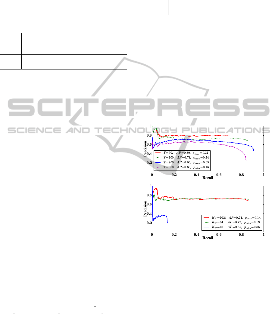
image classification accuracy. We learn the image
classification model on the train split of our dataset,
and report the average precision on both splits (train
and test) as well as the achieved overall sparsity. The
results are shown in Table 1.
Table 1: Influence of regularization and non-linear normal-
ization to the average classification precision.
R (w
w
w) normalization train sparsity test
L1 none 1.00 99.7% 0.72
L1 power + metric 0.91 99.6% 0.80
L2 none 1.00 0% 0.64
L2 power + metric 1.00 0% 0.73
Columns of the table correspond to the employed
regularizer (L1 or L2), applied regularization (either
only linear or linear, power and metric), AP on the
train split, the achieved sparsity of the classification
model, as well as the AP on the test split. The ta-
ble shows that L1 regularization succeeds to induce
classification models which employ only 0.3% (linear
normalization) and 0.4% (all normalizations) of the
Fisher vector representation. Even more interesting is
the fact that these sparse models outperform the stan-
dard dense models induced by L2 regularization by 8
(linear normalization) and 7 (all normalizations) per-
centage points of AP accuracy. Thus, it turns out that
by employing L1 normalization we are able to gain
both accuracy and efficiency. The table also shows
that some performance is lost by omitting nonlinear
normalizations: 8 (L1) and 9 (L2) percentage points.
However, this loss is not critical: we shall see that
the linear Fisher vector representation paired with the
sparse classification model shall achieve the weakly
supervised localization AP larger than the best classi-
fication AP from the Table 1.
Localization Baseline. In order to provide insight
into the difficulty of our problem, we show the re-
sults of a popular strongly supervised localization ap-
proach. We extract positive HOG descriptors (Dalal
and Triggs, 2005) at all groundtruth locations in the
train split, as well as about 25 times more nega-
tive HOG descriptors at random locations in a spe-
cial dataset containing many images without any
traffic signs. We used HOG implementation from
OpenCV library (Bradski, 2000). The parameters
of the HOG descriptor were: window size=(24,24),
block size=(4,4), block stride=(2,2), cell size=(2,2)
and n bins=9. We weight the training samples in or-
der to achieve class balance and learn a L2 regular-
ized logistic regression model. We apply the classifi-
cation model in the sliding window starting from the
size 24×24 at 64 scales, with a scale factor of 1.03
and achieve the results summarized in Table 2.
Table 2: Baseline localization results with a strongly su-
pervised linear classifier applied to HOG descriptors in the
sliding window.
AP train AP test processing time
results 0.968 0.944 10 s
Localization Results. We first evaluate the local-
ization performance when the patch scores are ob-
tained by using only soft-assign sparsity optimization.
The results are presented in the top panel of Figure
3. The method performs remarkably well, given the
difficulty of the problem. The best performance is
achieved when bounding boxes are derived from a
smaller number of top ranked patches T . However,
considering only a small number of highly ranked
patches increases the number of missed objects. In-
cluding more top ranked patches decreases the num-
ber of missed objects, but also deteriorates the detec-
tion performance.
Figure 3: Precision-Recall curves displaying localization
performance on the test set. Top: exploiting only soft-
assign sparsity with fixed K
SA
=4, full classification model
(K
W
=1024), and different numbers of top patches T to ob-
tain the bounding box candidates. Bottom: exploiting both
soft-assign sparsity (K
SA
=4) and model sparsity while vary-
ing the number (K
W
) of GMM components used by the
classification model and keeping the number of top patches
fixed (T =100). AP denotes the average precision and p
miss
corresponds to the proportion of missed objects (1-recall at
the rightmost datapoint).
Effects of the model sparsity optimization are
illustrated in the bottom panel of Figure 3. Our
discriminative model is very sparse: it has only
1277 non-zero coefficients, which corresponds to
only 0.77% of all image features. Consequently,
the performance drops only slightly when K
W
=64
VISAPP2015-InternationalConferenceonComputerVisionTheoryandApplications
50
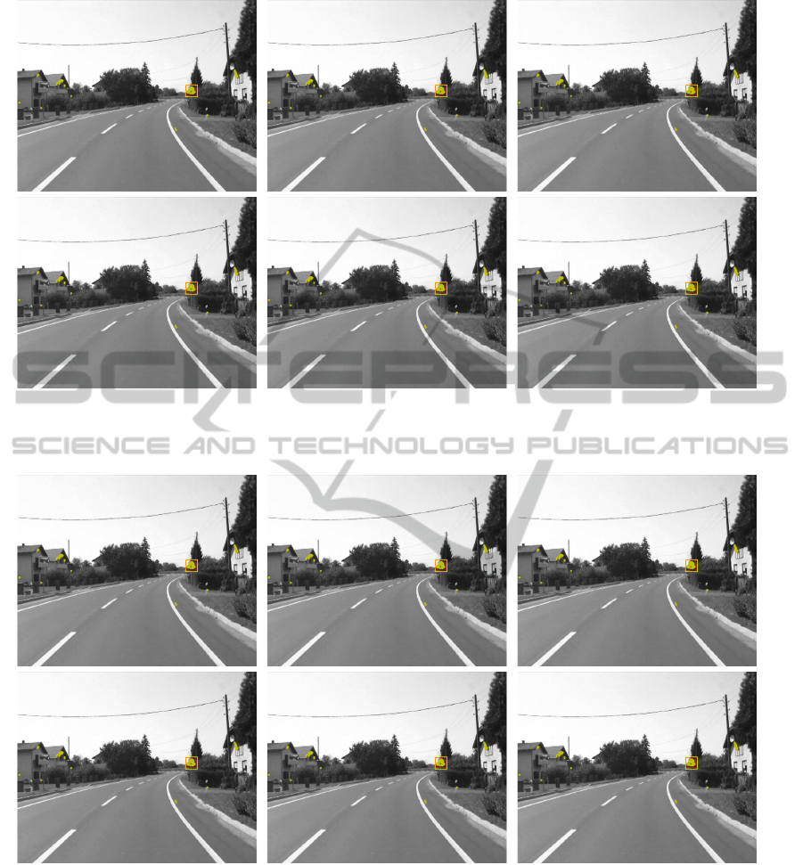
Figure 4: Successful operation: the method is able to detect multiple objects (cf . top-left) and to handle the complex back-
ground and small objects. Yellow dots indicate top ranked patches (rank< T ), yellow rectangles show the detected bounding
boxes, while red rectangles indicate the groundtruth locations (which are used exclusively for evaluation).
Figure 5: Detections counted as false alarms (top row), and missed detections (bottom row). The main causes of false alarms
are insufficient overlap with the groundtruth location and background structures similar to warning signs (e.g. roofs). Most
missed signs are either small or contain out-of-plane rotations which are seldom encountered in the train split.
top GMM components are employed. However, us-
ing as little as K
W
=16 top GMM components af-
fects performance significantly. The localization AP
on the train split was consistently better for 5 per-
cent points in experiments with K
W
=1024, K
SA
=4 and
T ∈ 50, 100, 200, 500. This means that the obtained
bounding boxes could be used to bootstrap the learn-
ing of strongly-supervised object detectors.
Figure 4 shows some examples of correctly de-
tected objects. The detected bounding boxes (yellow)
display very good overlap with the groundtruth loca-
tion (red). Note that we use the groundtruth location
exclusively for evaluation purposes, the training pro-
cedure knows only whether an image contains a warn-
ing sign or not.
Figure 5 shows two kinds of failure cases: bound-
WeaklySupervisedObjectLocalizationwithLargeFisherVectors
51

ing boxes with high scores that do not overlap with the
true bounding box, and true bounding boxes missed
by our detection method.
8 CONCLUSION AND
PERSPECTIVES
We have proposed a novel weakly supervised lo-
calization method based on classification of image
patches represented with large Fisher vectors. The
main advantage of our method is fast evaluation due
to a sparse linear classification model trained with L1
regularization. The sparsity of our model is deter-
mined by the parameter λ which regulates the trade-
off between the loss and the regularizer. We set that
parameter by cross-validation, which implies that our
model outperforms less sparse models on the train
split. Supplying a larger λ would lead to enhanced
sparsity and faster evaluation at the expense of some
performance loss.
To the best of our knowledge, this is the first ac-
count of patch Fisher vectors being used for weakly
supervised object localization. The method has
been experimentally validated on a challenging pub-
lic dataset and the obtained performance (90% recall,
75% precision) is comparable with strongly super-
vised approaches. The most interesting qualities of
the proposed approach include:
1. it is based on a slightly downgraded state-of-the-
art image classification approach;
2. does not require ad-hoc or bottom-up initializa-
tion;
3. it is trainable on images of very small objects (less
than 1% of the image content);
4. it is trainable on very large datasets (thousands of
images) in reasonable time.
Our results suggest that Fisher vectors hold a great
potential in the field of weakly supervised object lo-
calization. An interesting direction for future work
would be to use a block-sparse model to directly en-
force sparsity over GMM components. This would
also help to improve soft-assign time, which is cur-
rently the bottleneck of the method (our unoptimized
Python implementation takes around 20 s in the de-
tection stage). To this end we shall explore cascade
classifiers in the original feature space for quick re-
jection of the patches that can not contribute to the
top scores. An interesting extension would be a more
expressive spatial layout model for proposing bound-
ing boxes. Finally, we would like to tackle weakly-
supervised localization of fine-grained object classes,
as this problem has many interesting applications.
ACKNOWLEDGEMENTS
This work has been supported by the project VISTA
- Computer Vision Innovations for Safe Traffic,
IPA2007/HR/16IPO/001-040514 which is cofinanced
by the European Union from the European Regional
Development Fund.
Parts of this work have been performed while the
first author was funded by the European Commu-
nity Seventh Framework Programme under grant no.
285939 (ACROSS).
Parts of this work have been performed in the
frame of the Croatian Science Foundation project I-
2433-2014.
REFERENCES
Alexe, B., Deselaers, T., and Ferrari, V. (2010). What is an
object? In CVPR, pages 73–80.
Andrews, S., Tsochantaridis, I., and Hofmann, T. (2002).
”Support Vector Machines for Multiple-Instance
Learning”. In NIPS, pages 561–568.
Auer, P. (1997). ”On Learning From Multi-Instance Ex-
amples: Empirical Evaluation of a Theoretical Ap-
proach”. In ICML, pages 21–29.
Bach, F. R., Jenatton, R., Mairal, J., and Obozinski, G.
(2012). Optimization with sparsity-inducing penal-
ties. Foundations and Trends in Machine Learning,
4(1):1–106.
Bottou, L. (1991). ”Stochastic Gradient Learning in Neural
Networks”. In Neuro-N
ˆ
ımes.
Bradski, G. (2000). OpenCV library. Dr. Dobb’s Journal of
Software Tools.
Chen, Q., Song, Z., Feris, R., Datta, A., Cao, L., Huang,
Z., and Yan, S. (2013). Efficient maximum appear-
ance search for large-scale object detection. In CVPR,
pages 3190–3197.
Chum, O., Perdoch, M., and Matas, J. (2009). Geometric
min-hashing: Finding a (thick) needle in a haystack.
In CVPR, pages 17–24.
Chum, O. and Zisserman, A. (2007). An exemplar model
for learning object classes. In CVPR.
Cinbis, R. G., Verbeek, J. J., and Schmid, C. (2013). Seg-
mentation driven object detection with fisher vectors.
In ICCV, pages 2968–2975.
Cinbis, R. G., Verbeek, J. J., and Schmid, C. (2014). Multi-
fold MIL training for weakly supervised object local-
ization. In CVPR, pages 2409–2416.
Crandall, D. J. and Huttenlocher, D. P. (2006). ”Weakly
Supervised Learning of Part-Based Spatial Models for
Visual Object Recognition”. In ECCV, pages 16–29.
Crowley, E. J. and Zisserman, A. (2013). Of gods and
goats: Weakly supervised learning of figurative art. In
BMVC.
Csurka, G., Dance, C. R., Fan, L., Willamowski, J., and
Bray, C. (2004). Visual categorization with bags of
keypoints. In ECCV workshop, pages 1–22.
VISAPP2015-InternationalConferenceonComputerVisionTheoryandApplications
52

Dalal, N. and Triggs, B. (2005). ”Histograms of Oriented
Gradients for Human Detection”. In CVPR.
Deselaers, T., Alexe, B., and Ferrari, V. (2012). ”Weakly
Supervised Localization and Learning with Generic
Knowledge”. IJCV, 100(3):275–293.
Douze, M. and J
´
egou, H. (2009). Yael library.
https://gforge.inria.fr/projects/yael.
Everingham, M., Gool, L. J. V., Williams, C. K. I., Winn,
J. M., and Zisserman, A. (2010). ”The Pascal Visual
Object Classes (VOC) Challenge”. IJCV, 88(2):303–
338.
Felzenszwalb, P. F., Girshick, R. B., McAllester, D. A.,
and Ramanan, D. (2010). ”Object Detection with
Discriminatively Trained Part-Based Models”. PAMI,
32(9):1627–1645.
Galleguillos, C., Babenko, B., Rabinovich, A., and Be-
longie, S. J. (2008). ”Weakly Supervised Object Lo-
calization with Stable Segmentations”. In ECCV,
pages 193–207.
Gosselin, P.-H., Murray, N., J
´
egou, H., and Perronnin, F.
(2013). ”Inria+Xerox@FGcomp: Boosting the Fisher
vector for fine-grained classification”. Technical re-
port, INRIA.
Jaakkola, T. and Haussler, D. (1998). Exploiting generative
models in discriminative classifiers. In NIPS, pages
487–493.
Lampert, C. H., Blaschko, M. B., and Hofmann, T.
(2009). ”Efficient Subwindow Search: A Branch and
Bound Framework for Object Localization”. PAMI,
31(12):2129–2142.
Lowe, D. G. (2004). ”Distinctive Image Features from
Scale-Invariant Keypoints”. IJCV, 60(2):91–110.
Munder, S. and Gavrila, D. M. (2006). An experi-
mental study on pedestrian classification. PAMI,
28(11):1863–1868.
Nguyen, M. H., Torresani, L., la Torre, F. D., and Rother,
C. (2014). ”Learning discriminative localization
from weakly labeled data”. Pattern Recognition,
47(3):1523–1534.
Pandey, M. and Lazebnik, S. (2011). Scene recognition
and weakly supervised object localization with de-
formable part-based models. In ICCV, pages 1307–
1314.
Pedregosa, F., Varoquaux, G., Gramfort, A., Michel, V.,
Thirion, B., Grisel, O., Blondel, M., Prettenhofer,
P., Weiss, R., Dubourg, V., Vanderplas, J., Passos,
A., Cournapeau, D., Brucher, M., Perrot, M., and
Duchesnay, E. (2011). Scikit-learn: Machine learning
in Python. Journal of Machine Learning Research,
12:2825–2830.
Perronnin, F., S
´
anchez, J., and Mensink, T. (2010). ”Im-
proving the Fisher Kernel for Large-Scale Image Clas-
sification”. In ECCV, pages 143–156.
S
´
anchez, J., Perronnin, F., Mensink, T., and Verbeek, J. J.
(2013). ”Image Classification with the Fisher Vector:
Theory and Practice”. IJCV, 105(3):222–245.
Siva, P. and Xiang, T. (2011). ”Weakly supervised ob-
ject detector learning with model drift detection”. In
ICCV, pages 343–350.
Sivic, J. and Zisserman, A. (2003). Video google: A text
retrieval approach to object matching in videos. In
ICCV, pages 1470–1477.
Vedaldi, A. and Fulkerson, B. (2008). VLFeat: An open
and portable library of computer vision algorithms.
http://www.vlfeat.org/.
Viola, P. A. and Jones, M. J. (2004). ”Robust Real-Time
Face Detection”. IJCV, 57(2):137–154.
WeaklySupervisedObjectLocalizationwithLargeFisherVectors
53
