
Scalable and Iterative Image Super-resolution using DCT
Interpolation and Sparse Representation
Saulo R. S. Reis
1
and Graça Bressan
2
1
Dept. of Electrical Engineering, Federal University of Mato Grosso, UFMT, Cuiabá – Mato Grosso, Brazil
2
Dept. of Computing and Digital Systems Engineering, Polytechnic School of the University of São Paulo-EPUSP,
São Paulo-SP, Brazil
Keywords: Super-resolution, Sparse Representation, DCT Interpolation, k-SVD, OMP.
Abstract: In a scenario where acquisition systems have limited resources or available images do not have good
quality, super-resolution (SR) techniques are an excellent alternative for improving the image quality. The
traditional SR methods proposed in the literature are effective in HR image reconstruction to a
magnification factor up to 2. In recent years, example-based SR methods have shown excellent results in the
HR image reconstruction to magnification factor 3 or more. In this paper, we propose a scalable and
iterative algorithm for single-image SR using a two-step strategy with DCT interpolation and the sparse-
based learning method. The method proposed implements some improvements in the dictionary training and
the reconstruction process. A new dictionary is built by using an unsharp mask technique for feature
extraction. The idea is to reduce the learning time by using two different small dictionaries. The results were
compared with others interpolation-based and SR methods and demonstrated the effectiveness of the
algorithm proposed in terms of PSNR, SSIM and Visual Quality.
1 INTRODUCTION
Single-image super-resolution (SISR) method use
signal processing techniques to reconstruct a high-
resolution (HR) image from a set of low-resolution
(LR) images. When the acquisition systems have
limited resources or available images do not have
good quality, SR techniques are an excellent
alternative for improving the image quality.
Many important areas have benefited from SR
methods so far. In medicine, HR images are used to
help doctors to perform more accurate image
diagnosis. In remote sensing, HR images provide a
better interpretation and analysis of the sensed areas,
such as environmental, urban, agriculture, etc. In
surveillance systems, HR images can help the police
to identify suspects of vandalism or crimes. Other
areas that can benefit from high-quality content
include Digital TV, restoration of old content for
museums and libraries, etc.
SR methods adopt an observation model that
includes the effects of the acquisition process such
as optical distortion, blurring and noise.
This model can be described as:
=
+ (1)
where
of size =
×
pixels, represents the
observed LR image.
denotes the HR image of
size =
×
pixels, with >. Matrix of
size × represents the effects of the imaging
system, such as optical distortion and blurring.
Matrix represents the downsampling operator, and
is zero-mean white noise with variance
. The
fundamental SR problem is the recovery of HR
image
from the observed LR image
in (1)
without amplifying the effects of noise or blurring.
Traditional SR methods proposed in the
literature, such as interpolation-based (Zhang and
Xiaoling, 2006; Li and Orchard, 2001; Aly and
Dubois, 2005) and reconstruction-based (Park et al,
2003; Zibetti et al, 2011; Baker and Kanade, 2002),
have shown effective results in the HR image
reconstruction for magnification factors up to 2.
However, the image quality degrades rapidly for
upper magnification factors. One important
alternative to solve this problem is the use of
learning-based SR methods (Freeman et al., 2002;
Elad and Datsenko, 2009; Qiang et al., 2005; Jian et
al., 2003; Jiji and chaudhuri, 2006), that produce a
HR image by learning the co-occurrence patterns
between LR patches and their corresponding HR
patches.
463
Reis S. and Bressan G..
Scalable and Iterative Image Super-resolution using DCT Interpolation and Sparse Representation.
DOI: 10.5220/0005295304630470
In Proceedings of the 10th International Conference on Computer Vision Theory and Applications (VISAPP-2015), pages 463-470
ISBN: 978-989-758-089-5
Copyright
c
2015 SCITEPRESS (Science and Technology Publications, Lda.)

In the last years, many works have addressed the
learning-based methods based on the sparse
representation of signals. In these methods, each LR
image patch can be represented using a linear
combination of atoms from an overcomplete
dictionary. One of the pioneering works in this
direction was proposed by (Yang et al., 2010). Their
algorithm is divided into two main steps: a first step
of the Dictionary learning using LASSO and OMP
algorithms, and a second step of HR image
reconstruction. (Zeyde et al., 2010) also considered
a similar approach, but with some important
modifications. Their method adopted the use of the
k-SVD algorithm for dictionary learning and used a
pseudo-inverse expression for the HR dictionary
construction.
Some works have practiced the idea of using the
learning dictionary process according to the
structural content of LR and HR patches. In (Dong
et al, 2011), the Adaptive Sparse Domain Selection
– ASDS algorithm is used for selecting the patches.
In (Yang et al., 2012), the patches are grouped into
three different sets: soft patches, dominant
orientation patches and stochastic patches. In (Zhou
et al., 2012), the patches are divided using a Weber
Local Descriptor – WLD algorithm. The idea of
using a strategy of coupled dictionary training, is
presented in (Jia et al., 2013). The coupling is
carried out by forcing the sparse HR and LR patches
coefficients to have the same number of elements
different from zero.
Another emerging approach that has been
drawing research in recent years is image
interpolation based on DCT transform. (Wu et al.,
2010) proposed an Interpolation method for LR
video using a hybrid scheme with DCT transform
and Wiener filtering. The low frequency coefficients
are obtained by the DCT transform and the high
frequency coefficients by Wiener Filtering used in
the H.264/AVC standard. In this method, the filter
coefficients are calculated according to the images
of the training set. The SR method proposed in
(Garcia et al., 2012), applies DCT interpolation in
mixed-resolution videos based on multiple views of
the same scene. In (Hung et al., 2011) is proposed
the SR method, which the high-frequency
coefficients are retrieved using the adjacent high-
resolution frames (key-frames).
In this paper, we propose a scalable and iterative
single-image SR method. The algorithm is based on
a two-step strategy that uses the DCT interpolation
and sparse representation of signals.
The aim is to improve the high-resolution
reconstruction process, including the following
contributions:
• A new feature extraction step using an Unsharp
Mask in order to construct a new LR dictionary;
• Implementation of a scalable and iterative SR
process with the HR image obtained from the first
iteration, for a news two-step training and HR
reconstruction.
The remainder of this paper is organized as
follows. In section 2, sparse representation model
and DCT interpolation methods are revised. In
section 3, we detail the method proposed, composed
of two main steps. Experimental results are
presented in section 4 and we conclude this paper in
section 5.
2 BACKGROUND
2.1 Sparse Representation of Signals
In the sparse representation model, a natural signal
can be described as a sparse combination of atoms
with respect to an overcomplete dictionary, (Aharon
and Bruckstein, 2006). Given a signal ∈ℛ
and a
dictionary ∈ℛ
×
that contains k prototype
signal-atoms in columns, the sparsity-based
minimization problem is given by:
min
,
‖
−
‖
subjectto
‖
‖
≤
(2)
where
‖
.
‖
is the
norm,
‖
.
‖
is the
norm, is
a set of training signals,
is a sparse vector and
is target sparsity. Dictionary can be constructed
using a training process from a set of samples, or by
prespecified set of functions such as Fourier,
Wavelets and Curvelets (Aharon and Bruckstein,
2006). In the SR context, given a set of LR image
patches
=
{
}
, it can be represented as a
sparse combination with respect to LR dictionary
. In this case, the optimization problem is given
by:
arg
‖
−
‖
subjectto
‖
‖
≤
(3)
where (3) is minimized iteratively. First, we fix
and aim to find the best coefficients of matrix
according to the number of nonzero entries
. The
second step, the algorithm to search for a better
dictionary, according to updated sparse vectors
(Aharon and Bruckstein, 2006). An important
feature of the sparse representation model is the
possibility of using a reduced set of images
compared with traditional methods based on
learning examples.
VISAPP2015-InternationalConferenceonComputerVisionTheoryandApplications
464

2.2 Image Interpolation in the DCT
Domain
Image interpolation using DCT transform upscale
the image by adding coefficients of zero amplitude
in high frequency components of a block (Wu et al,
2010; Hung et al, 2011; Zhang and Chang, 2011;
Sun and Cham, 2007). The interpolation process
takes an important advantage of DCT domain, that
is, to concentrate the frequency coefficients values
in regions near the DC components.
First, a LR input image is divided into non-
overlapping blocks
of size ×. Then, for each
block
, a type II DCT transform is applied
resulting in a transformed block
()
as follows:
()
=
{
} (4)
Then,
()
is resized according to upscale
factor , by adding zeroes to high frequency
components, resulting in a
()
block as follows:
()
=
()
×
⋯0
⋮⋱⋮
0⋯0
×
(5)
Next, the inverse type III DCT transform is
applied to the resized block:
=
{
()
} (6)
where
is the resulting interpolated block of size
×.
3 PROPOSED SR METHOD
The proposed SR method is divided into two main
steps: a first step for training and construction of two
LR and HR dictionaries and a second step for
reconstructing the HR image, which will be detailed
in the sections 3.1 and 3.2.
In addition, we include a new section 3.3, which
addresses the iterative and scalable implementation
of the proposed method.
3.1 Step 1: Training and Dictionary
Construction
First, let a set of HR images of different features in a
set be blurred and downsampled, according to
equation (1), resulting in an equivalent set of LR
images.
For the construction of the LR dictionary
,
we used a set of four Laplacian and Gradient filters,
with the coefficients given by:
=
−1,0,1
,
=
,
=
1,0,−2,0,1
and
=
. These filters
are the same used in (Yang et al., 2010; Zeyde et al.,
2010). The feature extraction is performed according
to the following equation:
=
∗
(7)
where “ * ” denotes convolution operator,
is the
LR patch after the feature extraction process,
denotes the LR image of the training set and
(=1,2,3,4) represents the four Laplacian and
Gradient filters.
For dictionary
, we used an Unsharp Mask
(Gonzalez and Woods, 2010), as follows:
=
−
(
)
(8)
with,
(
)
=
∗
(9)
where
is low-pass filter and
(
)
is the
smoothed LR image. The idea of using the Unsharp
Mask is to extract features not present in dictionary
. The feature extraction with the unsharp mask
produces a new LR patch, given by:
=
∗
+.
(10)
where
represents an unsharp mask image and
is a weight to emphasize the contribution of the
unsharp mask. We adopt =1.
The use of the Laplacian and Gradient filters
produce LR patches
and
with high
dimensionality. In order to reduce the
dimensionality, the Principal Analysis Components
(PCA) algorithm is applied, using a projection
operator denoted by B. The resulting patches are
given by:
=
(11)
=
(12)
Considering LR patches
and
, the
dictionaries
and
are constructed using the
learning k-SVD and OMP algorithms (Aharon et
al., 2006), according to the following equations:
arg
−
subjectto
‖
‖
≤
(13)
arg
−
subjectto
‖
‖
≤
(14)
where
1
and
2
represent the sparse vectors with
respect to
1
and
2
and
is the target sparsity.
In order to reduce the learning time, dictionaries
and
are obtained by pseudo-inverse expression:
=
(15)
=
(16)
ScalableandIterativeImageSuper-resolutionusingDCTInterpolationandSparseRepresentation
465
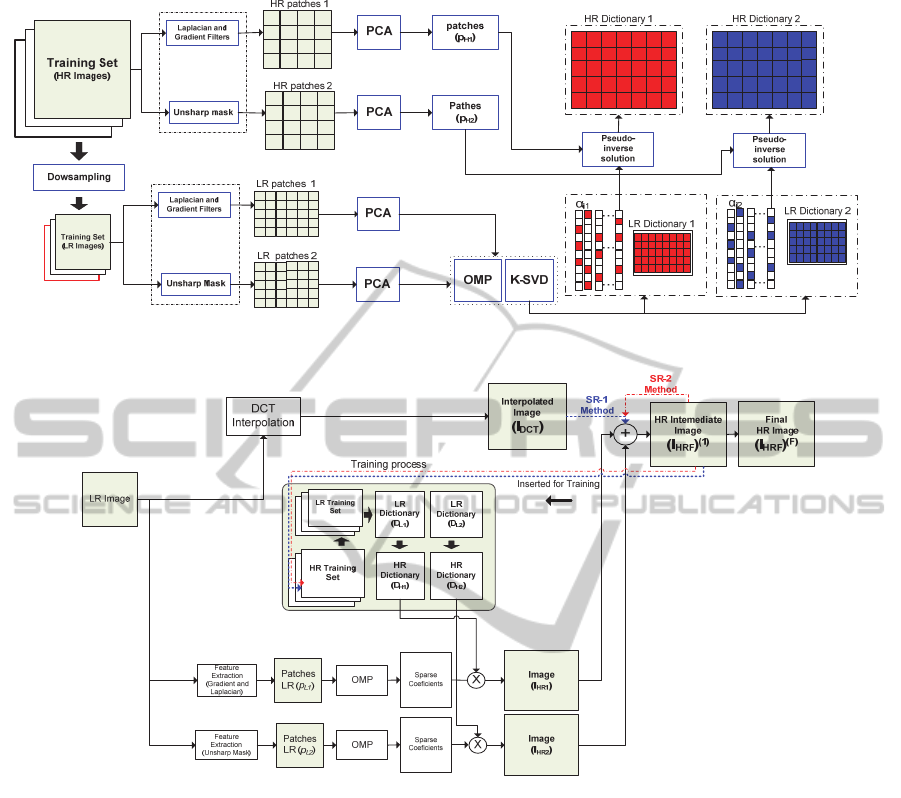
Figure 1: Overview of the Training and dictionary construction step described in section 3.1.
1i
α
2i
α
Figure 2: Framework of Iterative and scalable single-image SR method. In Both SR-1 and SR-2 implementation, The
(I
HRF
)
1
image is inserted in the training set for a new scalable and iterative process.
where
=1,2, represents the matrices built with
the HR patches extracted from the training set by
using (7) and (10).
and
are the matrices that
include all the vectors obtained in the sparse coding
process. Figure 1 shows an overall framework of
the proposed training and dictionary construction
step.
3.2 Step 2: HR Image Reconstruction
The HR image is reconstructed with the DCT-based
interpolated LR image and the other two images
obtained by sparse representation.
First, the input LR image
of size
×
pixels is interpolated with upscale factor using
DCT transform:
=
(17)
where
represents the interpolation operator in
the DCT domain described in section 2.2. Also, the
LR image
undergoes a feature extraction process
by high-pass filtering, using the same process
described in section 3.1. By applying this feature
extraction process, we get two different types of LR
patches, representing different features of the LR
image:
=
∗
(18)
=
∗
+.
(19)
Whereas
and
have high
dimensionality, we also used the PCA algorithm to
reduce the dimensionality, resulting in
and
patches. Given
,
,
and
, the
proposed algorithm uses a sparse coding algorithm
VISAPP2015-InternationalConferenceonComputerVisionTheoryandApplications
466

OMP to calculate the sparse coefficients
and
, according to equations (13) and (14).
Considering sparse coefficients
and
, the
HR patches are obtained by:
=
(20)
=
(21)
Patches
and
are combined with a least
squares solution to obtain partial images
and
:
=
∑
∑
(22)
=
∑
∑
(23)
The HR final image consists in the interpolated
image DCT
and the two images obtained by
the learning process
and
:
(
)
=
+
(
+
)
(24)
where is a factor that represents the contribution of
learning Images. In this paper, we adopt =1/2.
A
framework of the proposed SR method is presented
in Figure 2.
3.3 Scalable and Iterative
Implementation
An important contribution of the proposed method is
to combine step 1 and step 2 in a scalable and
iterative way. The partial HR image
(
)
obtained in
the first iteration is inserted into the training set to
run a new training step. In this case, the final HR
image is given by:
(
)
=
(
)
+
(
)
+
(
)
,
n=2,…,N
(25)
where is the number of iterations of the algorithm.
The HR image of the first iteration can be inserted in
the training set of two ways:
• In the first case, the
(
)
image is constructed
with the same upscale factor of the final HR
image. This image is inserted in the training set
for a new step of dictionary training. This case
was tested for upscale factor up to 2.
• In the second case, the
(
)
image is constructed
with an upscale factor smaller than final HR
image. This image is inserted in the training set
for a new of dictionary training. The high
frequency coefficients recovered in
(
1
)
image
are transformed into low frequency coefficients
in the next iteration of algorithm. For the
simulations tests in section 4, we used an upscale
factor 3 to final HR image.
4 EXPERIMENTAL RESULTS
4.1 Simulations Settings
To illustrate the performance of the proposed
algorithm, computer simulations were performed in
MATLAB
®
using a computer with Intel Dual Core
T4300 2.10 GHz, 3 GB RAM. The images used for
the tests were Cameraman, Jetplane, Lake, Lenna
and Living Room. These images were degraded by
blurring and subsampling and then upscaled using
factors equal to 3. For training and construction of
the LR dictionaries, we used 20 iterations of k-SVD
and OMP algorithms. The training set used for the
training step, was the same used in (Yang et al,
2010; Zeyde et al, 2010), composed by 92 images
that include flowers, landscapes, faces, buildings, in
order to extract different features such as edges and
textures. However, for the proposed SR algorithm
was used only 5 images of the training set.
Apart from inclusion of the HR image in the
training set as described in section 3.3, in all
simulations, we adopted two configurations for the
reconstruction step:
a) SR-1 algorithm: the intermediate image
(
)
was
replaced by the interpolated image
to perform
one more iteration of algorithm. This configuration
is denoted in Table 1 as SR-1.
b) SR-2 algorithm: the intermediate image
(
)
is
updated for each iteration of algorithm. This
configuration is denoted in Table 1 as SR-2.
The proposed algorithms SR-1 and SR-2 was
compared with interpolation-based methods such as
bicubic and DCT interpolation, and SR methods
proposed in (Yang et al, 2010) and (Zeyde et al,
2010).
4.2 Results
Table 1 shows the results in terms of PSNR and
SSIM of proposed SR-1 and SR-2 algorithms
compared with others SR methods. We can observe
that the SR-2 algorithm produced superior results
than all others methods. The results indicate that the
scalable and iterative strategy using few images of
the training set was efficient in the process of
reconstruction of HR final image
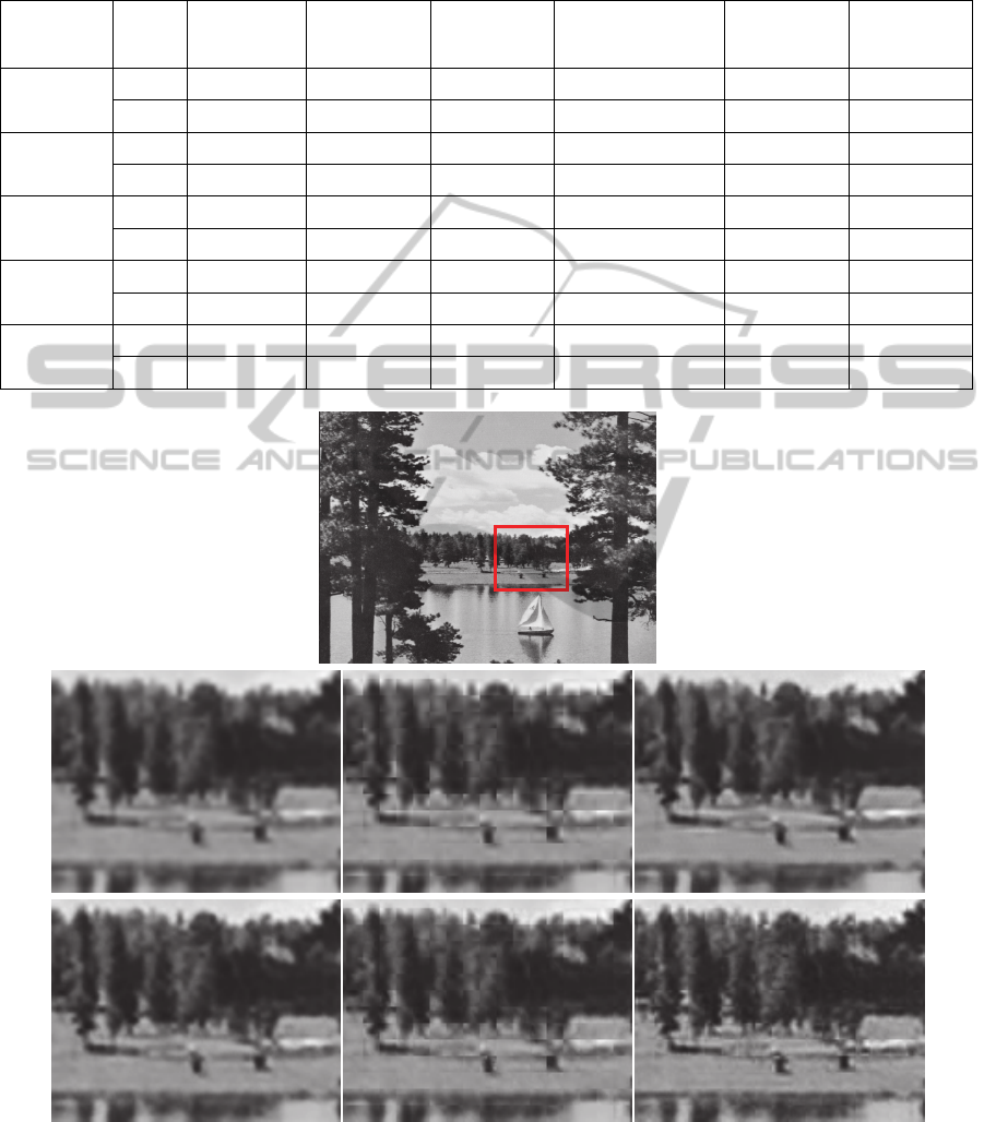
Figures 3 and 4 show the results of the SR-1
and SR-2 algorithms, considering the quality visual
ScalableandIterativeImageSuper-resolutionusingDCTInterpolationandSparseRepresentation
467

of the HR image obtained by the methods. We can
observe in figures 3(g) and 4(g), that the proposed
algorithm SR-2 has recovered more details than
others methods. In addition, we observe a
minimization of the blocking effects caused by DCT
interpolation in the proposed method SR-2.
5 CONCLUSIONS
In this paper, we proposed a novel scalable and
iterative single-image SR method using DCT
interpolation and sparse representation. The
proposed method uses a training strategy of two
dictionaries with different high-pass filters to feature
extraction and a reduced training set.
Computer simulations demonstrated the
effectiveness of the proposed method in terms of
PSNR, SSIM and visual quality.
REFERENCES
Aharon, M., Elad, M., Bruckstein, A., 2006. K-SVD: An
algorithm for designing overcomplete dictionaries for
sparse representation. IEEE Transactions on Signal
Processing, vol. 54, no. 11, pp. 4311-4322.
Aly H. A., Dubois E., 2005. Image Up-Sampling Using
Total-Variation Regularization with a New
Observation Model. IEEE Transactions on Image
Processing, vol. 14, no. 10, pp. 1647-1659.
Baker, S., Kanade, T., 2002. Limits on super-resolution
and how to break them. IEEE Transactions on
Pattern Analysis and Machine Intelligence, vol. 24,
no. 9, pp. 1167-1183.
Dong, W., Zhang, L., Shi, G., 2011. Image Deblurring and
Super-Resolution by Adaptive Sparse Domain
Selection and Adaptive Regularization. IEEE
Transactions on Image Processing, vol. 20, no. 7, pp.
1838-1857, Jul, 2011.
Elad, M., Datsenko, D., 2009. Example-Based
Regularization Deployed to Super-Resolution
Reconstruction of a Single Image. Computer Journal,
vol. 52, no. 1, pp. 15-30.
Freeman, W. T., Jones, T. R., Pasztor, E. C., 2002.
Example-based super-resolution. IEEE Computer
Graphics and Applications, vol. 22, no. 2, pp. 56-65,
Mar-Apr.
Garcia, D. C., Dorea, C., Queiroz, R. L., 2012. Super
Resolution for Multiview Images Using Depth
Information. IEEE Transactions on Circuits and
Systems for Video Technology, vol. 22, no. 9, pp.
1249-1256.
Gonzalez, R. C., Woods, R. E., 2010. Digital Image
Processing, Pearson, Third Edition.
Hung, E. M., Garcia, D.C., Queiroz, R.L.D., 2011.
Transform domain semi-super resolution. in ICIP'11,
pp. 1193-1196.
Jia, K. , Wang, X. , Tang, X., 2013. Image Transformation
Based on Learning Dictionaries across Image Spaces.
IEEE Transactions on Pattern Analysis and Machine
Intelligence, vol. 35, no. 2, pp. 367-380.
Jian, S., Nan-Ning, Z., Hai, T., 2003. Image hallucination
with primal sketch priors. Proceedings. 2003 IEEE
Computer Society Conference on Computer Vision
and Pattern Recognition. pp. II-729-36 vol.2.
Jiji, C. V. Chaudhuri, S., 2006. Single-frame image super-
resolution through contourlet learning. Eurasip
Journal on Applied Signal Processing, 2006.
Li X., Orchard M., 2001. New Edge-Directed
Interpolation. IEEE Transactions on Image
Processing. vol. 10, no. 10, pp. 1521-1527.
Park, S. C., Park, M. K., Kang, M. G., 2003. Super-
resolution image reconstruction: A technical overview.
IEEE Signal Processing Magazine, vol. 20, no. 3, pp.
21-36.
Qiang, W., Xiaoou, T., Shum, H., 2005. Patch based blind
image super resolution. Tenth IEEE International
Conference on Computer Vision, 2005. ICCV 2005,
pp. 709-716 Vol. 1.
Sun, D., Cham, W. K., 2007. Postprocessing of low bit-
rate block DCT coded images based on a fields of
experts prior.
IEEE Transactions on Image
Processing, vol. 16, no. 11, pp. 2743-2751.
Wu, Z., Yu, H., Chen, C. W., 2010. A New Hybrid DCT-
Wiener-Based Interpolation Scheme for Video Intra
Frame Up-Sampling. IEEE Signal Processing Letters,
vol. 17, no. 10.
Yang, J., Wright, J., Huang, T. S., 2010. Image Super-
Resolution Via Sparse Representation. IEEE
Transactions on Image Processing, vol. 19, no. 11.
Yang, S., Wang M., Chen Y., 2012. Single-Image Super-
Resolution Reconstruction via Learned Geometric
Dictionaries and Clustered Sparse Coding. IEEE
Transactions on Image Processing, vol. 21, no. 9, pp.
4016-4028.
Zeyde R., Elad, M., Protter, and M. 2010. On single image
scale-up using sparse-representations. Proceedings of
the 7th international conference on Curves and
Surfaces. pp 711-730.
Zhang, W., Cham, W. K., 2011. Hallucinating Face in the
DCT Domain. IEEE Transactions on Image
Processing, vol. 20, no. 10, pp 2769-2779.
Zhang L., Xiaoling W., 2006. An Edge-Guided Image
Interpolation Algorithm via Directional Filtering and
Data Fusion. IEEE Transactions on Image
Processing, vol. 15, no. 8, pp. 2226-2238.
Zhou F., Yang, W. Liao, Q., 2012. Single Image Super-
Resolution Using Incoherent Sub-dictionaries
Learning. IEEE Transactions on Consumer
Electronics, vol. 58, no. 3, pp. 891-897.
Zibetti, M. V. W., Bazan, F. S. V. Mayer, J., 2011,
Estimation of the parameters in regularized
simultaneous super-resolution. Pattern Recognition
Letters, vol. 32, no. 1, pp. 69-78.
VISAPP2015-InternationalConferenceonComputerVisionTheoryandApplications
468
APPENDIX
Table 1: PSNR and SSIM Results for upscale 3 and 20 iterations of k-SVD and OMP algorithms.
Image Metric
Bicubic
Interpolation
DCT
Interpolation
SR Method
(YANG et al.,
2010)
SR Method
(ZEYDE et al., 2010)
Proposed
Method SR-1
Proposed
Method SR-2
Cameraman
PSNR 30.367 30.299 32.018 32.620 32.0563
33.987
SSIM 0.9587 0.9640 0.959 0.974 0.969
0.984
Jetplane
PSNR 29.429 29.313 30.383 30.980 29.976
31.311
SSIM 0.957 0.961 0.956 0.971 0.965
0.968
Lake
PSNR 27.419 27.414 28.063 28.556 27.917
29.599
SSIM 0.938 0.937 0.944 0.956 0.949
0.971
Lenna
PSNR 31.704 31.622 32.668 33.029 33.436
33.565
SSIM 0.953 0.958 0.956 0.966 0.970
0.977
Living Room
PSNR 26.840 26.834 27.441 27.608 27.327
28.537
SSIM 0.893 0.904 0.912 0.920 0.914
0.956
Figure 3: Visual quality results for Lake Image
(
512×512
)
pixels, considering upscale factor of 3 and dictionary size of
512. (a) Original image, (b) Bicubic interpolation, (c) DCT interpolation, (d) SR method proposed in Yang et al (2010) (e)
SR method proposed Zeyde et al (2010), (f) Our method SR-1 and (g) Our method SR-2.
(
a
)
(
b
)
(
c
)
(
d
)
(
e
)
(
f
)
(g)
ScalableandIterativeImageSuper-resolutionusingDCTInterpolationandSparseRepresentation
469
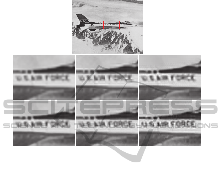
Figure 4: Visual quality results of Jet plane image
(
512×512
)
pixels, considering upscale factor of 3 and dictionary size
of 512. (a) Original Image, (b) Bicubic interpolation, (c) DCT interpolation, (d) SR method Yang et al (2010) (e) SR
method Zeyde et al (2010), (f) Our method SR-1 and (g) Our method SR-2.
(
a
)
(
b
)
(
c
)
(
d
)
(
e
)
(
f
)
(g)
VISAPP2015-InternationalConferenceonComputerVisionTheoryandApplications
470
