
SIFT-EST
A SIFT-based Feature Matching Algorithm using Homography Estimation
Arash Shahbaz Badr, Luh Prapitasari and Rolf-Rainer Grigat
Institute of Vision Systems, Hamburg University of Technology, Harburger Schlossstrasse 20, Hamburg, Germany
Keywords:
Image Correspondences, Feature Matching, Local Features, SIFT, Homography Estimation.
Abstract:
In this paper, a new feature matching algorithm is proposed and evaluated. This method makes use of features
that are extracted by SIFT and aims at reducing the processing time of the matching phase of SIFT. The idea
behind this method is to use the information obtained from already detected matches to restrict the range
of possible correspondences in the subsequent matching attempts. For this purpose, a few initial matches
are used to estimate the homography that relates the two images. Based on this homography, the estimated
location of the features of the reference image after transformation to the test image can be specified. This
information is used to specify a small set of possible matches for each reference feature based on their distance
to the estimated location. The restriction of possible matches leads to a reduction of processing time since the
quadratic complexity of the one-to-one matching is undermined. Due to the restrictions of 2D homographies,
this method can only be applied to images that are related by pure-rotational transformations or images of
planar object.
1 INTRODUCTION
Finding correspondences between multiple views of
the same scene or object is a key component of var-
ious computer vision and robotics applications, such
as camera calibration, image stitching, automated 3D
modeling, motion tracking, and many more. A cor-
respondence is given by image points that depict the
same physical point in different images. Such corre-
spondences can be found by the help of local image
features. Local features hold some distinctive infor-
mation on the visual content of a relatively sparse set
of distinguished image regions.
The process of finding image correspondences can
be divided into three steps: feature extraction, fea-
ture description and feature matching. The feature
extraction step explores an image to detect distinc-
tive features. The distinctiveness of features allows
for locating them in different views. The feature de-
scription step captures some information on the local
appearance of the detected features. This information
is stored in a feature descriptor, which is a vector of
fixed size. In order to find correspondences, the fea-
ture descriptors of a reference image are compared to
those of a test image. This comparison is done in the
feature matching step.
The matches between image features are de-
termined by a similarity measure. Therefore, the
changes in the appearance of the images disturb the
matching process. Images that are involved in fea-
ture matching are related by different photometric
and geometric transformations, such as illumination
change, blur, zooming, camera translation, and rota-
tion. These transformations modify, among others,
the shape, scale, position, and orientation of the de-
picted scene objects in the image. Moreover, due to
these transformations, some objects may get occluded
by others or may be moved out of the visible frame.
The challenge is to design extraction, description, and
matching algorithms that are invariant or, at least to
some extent, robust against such distortions.
This paper proposes a feature matching method
based on the well-known SIFT-Method. With this ap-
proach, the computational cost of the matching step
of SIFT can be reduced significantly. The proposed
method utilizes a small set of initial matches in order
to estimate the transformed position of the reference
features and restrict the set of possible test features
for the following matching attempts. The estimation
is based on the homography that defines the transfor-
mation between the two images. The homography do
not cover the general transformation. Therefore, the
application of the proposed method is limited to two
specific scenarios. First scenario is when the images
504
Shahbaz Badr A., Prapitasari L. and Grigat R..
SIFT-EST - A SIFT-based Feature Matching Algorithm using Homography Estimation.
DOI: 10.5220/0005296105040511
In Proceedings of the 10th International Conference on Computer Vision Theory and Applications (VISAPP-2015), pages 504-511
ISBN: 978-989-758-091-8
Copyright
c
2015 SCITEPRESS (Science and Technology Publications, Lda.)

are captured by cameras that have a common center
of projection. This means that the cameras are related
by pure rotation around the optical center (no transla-
tion). The second scenario is when all image points
lie on the same plane in the scene. Possible applica-
tions are, for instance, generating panorama images
and optical text recognition.
The remainder of this paper is organized as fol-
lows. Section 2 gives an overview of some of the
popular existing methods. Section 3 briefly reviews
the SIFT method. Section 4 describes the proposed
method. Section 5 evaluates the proposed method
by representing the experimental results. And finally,
Section 6 concludes this paper.
2 RELATED WORK
There exists a wide variety of approaches for finding
correspondences between digital images. Some ap-
proaches provide a framework for the whole process
(extraction, description, and matching), while others
introduce novel methods for specific steps and use ex-
isting methods for the others. In this section, some of
the most popular methods are introduced.
Harris corner detector (Harris and Stephens, 1988)
is a relatively simple, though widely-used feature de-
tector. This method searches for points with sig-
nificant signal changes in two orthogonal directions.
Such points correspond mostly to physical corners
in the scene. The detection is done by observing a
self-similarity measure while shifting a small window
around a point. The biggest weakness of the Harris
method is the lack of scale invariance.
SIFT (Lowe, 2004) is one of the most prominent
approaches. SIFT features provide scale and rota-
tion invariance in addition to partial illumination and
affine invariance. These strengths come at the price
of high computational complexity, mainly caused by
scale-space processing and high dimensionality of de-
scription vectors. Furthermore, the matching accu-
racy drops drastically in case of changes higher than
about 30 degrees in viewpoint angle (affine transfor-
mation). Nevertheless, due to its solid performance,
SIFT has become a supposed standard for finding im-
age correspondences.
Due to the strengths of SIFT, numerous varia-
tions have been proposed in the recent decade to over-
come its shortcomings. ASIFT (Yu and Morel, 2011),
for instance, extends SIFT with full affine-invariance
by applying various tilts and rotations to the image
to simulate different camera orientations. After the
viewpoint simulation, ASIFT follows the standard
SIFT method. Although ASIFT outperforms SIFT in
scenarios with high viewpoint changes, the complex-
ity caused by the preprocessing increases the compu-
tation time considerably (Wu et al., 2013). PCA-SIFT
(Ke and Sukthankar, 2004) is another SIFT-variant,
which aims at reducing the computational complexity.
This method utilizes the Principle Component Anal-
ysis (PCA) to reduce the descriptor dimension. The
compact descriptor declines the matching time, but
the PCA-processing introduces further costs in the de-
scription step. The overall processing time is reduced
slightly, but the performance is compromised in some
cases (Mikolajczyk and Schmid, 2005), (Wu et al.,
2013). SURF (Bay et al., 2008) is a further approach
that reduces the complexity of SIFT. The lower com-
plexity is due to rough approximations and reduced
descriptor size. SURF has shown to improve the com-
putation efficiency of SIFT significantly while achiev-
ing comparable accuracy (Bay et al., 2008), (Grau-
man and Leibe, 2011), (Wu et al., 2013).
Affine invariant region detectors (Mikolajczyk
and Schmid, 2002), (Mikolajczyk and Schmid, 2004)
achieve limited affine-invariance by iteratively esti-
mating and normalizing the local affine shape of the
features. However, due to the fact that the features are
extracted in a non-affine manner, full affine invariance
cannot be achieved (Lowe, 2004).
Lepetit and Fua (Lepetit and Fua, 2006) redefine
the feature matching problem as a classification prob-
lem, where the features of the reference image are
considers as classes and the features of the test image
are classified based on their appearance. The classifier
is trained by applying random affine transformations
to the reference image to simulate different views of
each feature. The features are matched (classified) in
real-time using randomized trees. With this scheme,
the computational complexity is moved to the extrac-
tion (training) step to enable fast matching phase.
3 REVIEW OF SIFT
As mentioned before, the proposed method is based
on the SIFT approach. Therefore, this section
presents a short review of the different steps of this
method based on (Lowe, 2004).
3.1 Feature Extraction
In order to achieve scale invariance, SIFT exploits
the concept of the scale space, which builds a
3-dimensional space by enhancing the image space
with scale. For this purpose, the image is smoothed
successively with the scale-normalized Gaussian ker-
nel. Each blurred image represents one instance of the
SIFT-EST-ASIFT-basedFeatureMatchingAlgorithmusingHomographyEstimation
505

scale space. The complete scale space is constructed
by successive application of Gaussian filters of vary-
ing scales.
For detecting the features, the Difference-of-
Gaussian function (DoG) is convolved with the im-
age. The DoG is the subtraction of two Gaussian
functions that are separated by a constant scale factor.
Therefore, the convolution is equivalent to subtrac-
tion of two adjacent scale-space levels. The potential
features are localized at the local extrema of the com-
puted subtractions in scale and space.
The detected feature candidates are discrete with
respect to scale and space. Hence, they may not be
located at the actual extrema of the DoG function. In
order to achieve a sub-pixel and sub-scale precision, a
3D fitting is performed. In the last step, low-contrast
points and points along edges are discarded due to
their instability.
3.2 Feature Description
An important property of SIFT-features is their rota-
tion invariance. This property is achieved by gener-
ating the descriptors relative to the local orientations
of the features. For this purpose, the gradient magni-
tudes and orientations of the pixels around each fea-
ture are computed. The gradient orientations are then
weighted with the respective gradient magnitudes and
a Gaussian window. Subsequently, for each feature a
36-bin histogram of the weighted orientations is gen-
erated corresponding to 360 degrees. The peaks of the
histograms determine the orientations of the features.
For a distinctive description, a 16 × 16 pix-
els patch around each feature is divided into sixteen
4 × 4 subregions. For each subregion, a histogram of
weighted orientations is built. Each histogram con-
sists of 8 bins, which gives rise to 16 × 8 = 128 el-
ements in the descriptor vector. To reduce the sensi-
tivity to illumination changes, the descriptor is lastly
normalized.
3.3 Feature Matching
For finding matching features in different images,
SIFT utilizes a ratio threshold that checks the gap be-
tween the best match and the second best match. The
best and second best matches are given by the two
nearest neighbors of the feature considering the Eu-
clidean distances of the descriptor vectors. Suppose
that the descriptor of a reference feature has the Eu-
clidean distances d
1
and d
2
to its first and second near-
est neighbors in the test image. If the ratio
d
1
d
2
is lower
than a predefined threshold, the nearest neighbor is
chosen as the matching feature, otherwise no match
is assigned to the feature. This approach outperforms
a simple distance thresholding approach since it can
discard indistinctive matches independent of the ac-
tual distance d
1
.
The one-to-one matching of features has a
quadratic complexity in the number of detected fea-
tures. Moreover, it has been shown that no search al-
gorithm exists that performs better than the exhaustive
search in spaces with dimensions higher than about
ten (Lowe, 2004), (Mount, 1998). To ensure a practi-
cable implementation, SIFT exploits a priority search,
called Best-Bin-First (BBF), which provides an in-
dexing scheme based on the distance of the nodes
to the query. The search is stopped after 200 nodes
have been checked. BBF is an approximating algo-
rithm that returns the exact nearest neighbor with high
probability or a close neighbor in other cases. This
approach gives rise to considerable reduction of pro-
cessing time for images with high number of features.
4 PROPOSED METHOD
The proposed method is dubbed SIFT-EST, which
stands for pre-estimated matching of SIFT features.
Figure 1 shows the block diagram of the method. As
implied by the diagram, SIFT-EST makes use of fea-
tures that are extracted and described by the SIFT
method, and differs from SIFT in the matching phase.
The matching step is divided into an initial matching
step, followed by homography estimation and final
matching. The initial matching finds a small subset of
correspondences. These correspondences are utilized
to estimate the homography that defines the transfor-
mation between the two images. The estimated ho-
mography is then used to roughly estimate the posi-
tion of the reference features in the test image. In
the final matching step, for each reference feature a
set of relevant test features are specified. A test fea-
ture is relevant for a reference feature if it is located
within a predefined radius from the estimated location
of the transformed reference feature. Subsequently,
the reference features are matched only against the
relevant test features. With this scheme, the quadratic
complexity of the exhaustive search is undermined
since the reference features are only matched against
a small fraction of test features. The three steps of
the proposed matching scheme are elaborated in the
following subsections.
4.1 Initial Matching
After feature extraction and description, the initial
matching step finds a predefined number of matches.
VISAPP2015-InternationalConferenceonComputerVisionTheoryandApplications
506

Feature Extraction (SIFT)
Feature Description (SIFT)
Homography Estimation
Initial Matching
Final Matching
Figure 1: The block diagram of the proposed method.
The matching is iterated until enough matches are
found, or all reference features have been checked.
The matching procedure is similar to SIFT, however
the order of selecting features differs. In SIFT, the
reference features are matched according to the order
in which they are extracted. This order is based on the
location of features in the image. The initial match-
ing step finds only a small subset of correspondences.
Following this order would result in matches that are,
with high probability, very close to each other or even
overlapping. In this case, the homography estimation
would possibly fail to find a proper transformation.
For this reason, SIFT-EST chooses the reference fea-
tures randomly. The drawback of this scheme is that
the deterministic behavior of SIFT is lost since differ-
ent sets of initial matches can result in different re-
sults.
Since the initial matches specify the homography
and, consequently, affect the performance, their ac-
curacy is of utmost importance. Therefore, the ra-
tio threshold used in the initial matching step has to
be set relatively low to suppress the chance of mis-
matches. Considering the empirical observations in
(Lowe, 2004), a ratio threshold of 0.25 has been cho-
sen, which provides a nearly-zero probability of in-
correct matches.
4.2 Homography Estimation
The initial matches found previously are utilized to
estimate the transformation between the two images.
The proposed method makes use of the 2D homogra-
phy, H, to relate the images. The respective transfor-
mation of image points is defined as:
x
2
= Hx
1
, (1)
where H is a 3 × 3 transformation and x
1
, x
2
denote
the homogeneous coordinates of two corresponding
points in the first and second image.
To ensure fast processing, the estimation is carried
out by a simple, linear method called normalized DLT
(Direct Line Transformation) as described in (Hart-
ley and Zisserman, 2004). The homography has eight
degrees of freedom (one less than the number of el-
ements due to scale ambiguity of homogeneous co-
ordinates). Each point correspondence generates two
linear equations constraining the x and y coordinates.
Hence, only four correspondences are sufficient for
the estimation. However, using the minimum number
of initial matches often results in inaccurate estima-
tions. For the experiments of this paper, the number
of initial matches is set to six, which showed reason-
able results at low cost.
4.3 Final Matching
Once the homography is estimated, it is used to esti-
mate the position of the reference features in the test
image. For this purpose, all reference features that
have not been involved in the initial matching step
are mapped to the second image based on the homog-
raphy. For each reference feature, the relevant test
features are determined by checking the distance of
all test features form the respective mapped location.
Test features that are within a predefined radius from
the mapped location are considered for the matching.
Figure 2 illustrates this scheme.
H
Figure 2: Specifying relevant features. The line visualizes
the mapping of a feature of the reference image to the test
image using the estimated homography. The circle deter-
mines the relevant test features based on their distance to
the mapped location. The points indicate the location of all
test features.
The radius should be large enough to count for
the estimation error. The experiments use a radius of
50 pixels. This value may seem large, but the area that
is covered by this circle is much smaller than the com-
plete image area. For instance, in an image with the
resolution of 765 × 512 pixels (smallest image used
in the experiments) this circle covers only 2% of the
area of the image. Respectively, the number of fea-
tures within this circle is relatively small.
After finding the relevant test features, the match-
ing process is similar to the standard matching
method of SIFT. The difference is that the ratio
thresholding is followed by a distance thresholding.
SIFT-EST-ASIFT-basedFeatureMatchingAlgorithmusingHomographyEstimation
507

The strength of the ratio threshold in SIFT is due to
the dense set of test features. However, here exists
only a small number of relevant test features or even
a single one. Thus, the ratio threshold alone cannot
determine the distinctiveness of the matches. There-
fore, a distance threshold is required to check if the
respective features are indeed similar. Furthermore,
the experiments showed that applying a sole distance
threshold declines the performance slightly. Hence,
the combination of both thresholds is implemented.
The additional cost introduced by applying the second
threshold is minimal since the descriptor distances are
already computed for the first thresholding procedure.
5 EVALUATION
In this section, the proposed method is evaluated. For
this purpose, the accuracy and processing time of
SIFT-EST is compared to SIFT to see if the expected
improvements are achieved. Before presenting the re-
sults, the procedure of the experiments and the eval-
uation measures are described to make the respective
results reproducible.
5.1 Experimental Setup
All the experiments are run on a PC with Intel Core
i5-4670@3.40 GHz processor and 16 GB memory
running 64-bit Windows 7. The experiments are im-
plemented and executed with Matlab 2013b. Beside
the scripts that are implemented to execute and evalu-
ate the experiments, additional toolboxes or functions
have been utilized, which are discussed here.
For extraction, description and matching of SIFT
features, the VLFeat
1
library version 0.9.17 is used.
The features are extracted and described using the de-
fault parameters given by the author of SIFT. For the
matching step a ratio threshold of 0.5 is used. Please
note that the VLFeat library uses the inverse of the
threshold proposed by Lowe. Therefore, the actual
input of the respective SIFT-function is set to 2.
The SIFT-EST method differs from SIFT in the
matching step. Hence, the Feature extraction and de-
scription are performed with the respective functions
from the VLFeat library. In the initial matching phase,
the call to the matching function has been modified to
change the order of matching attempts as discussed
in 4.1. The ratio threshold used in this phase is 0.25.
The homography estimation is performed by the help
of the Homography Estimation Toolbox
2
with six pu-
tative correspondences. In the final matching phase, a
1
www.vlfeat.org
2
www.it.lut.fi/project/homogr
ratio threshold of 0.5 is used. The ratio thresholding
is followed by an additional distance thresholding as
discussed in 4.3.
For the experiments, four sets of images have been
used, which are distributed by the Visual Geometry
Group (VGG) of the Oxford University
3
and are fre-
quently used in literature for the evaluation of fea-
ture extraction, description and matching algorithms.
These sets are chosen since all images either depict
planar scenes or are captured without camera trans-
lation. Therefore, they comply with the proposed
method. Two sets (Graf and Wall) contain viewpoint
changes ranged from a fronto-parallel view to one at
approximately 60 degrees relative to the camera. The
other two sets (Bark and Boat) represent combina-
tions of rotation and scale changes. The scaling is
obtained by varying the camera zoom. The rotation
changes are produced by rotating the camera around
its optical axis (Z-direction) between 30 and 45 de-
grees. Figure 3 shows one image of each set.
Figure 3: Four sets from the VGG database are used for the
experiments. Set names from left to right: Bark, Boat (top),
Graf, and Wall (bottom).
Each set contains six images, where the first input
image is used as the reference for the other five. For
each set, five homographies are provided as ground
truth that define the geometric transformations rel-
ative to the reference image. Using these homo-
graphies, the accuracy of the methods can be deter-
mined with the following procedure. After applying
a feature matching algorithm, the matched reference
features are transformed to the respective test image
based on the provided homography. Subsequently, the
spatial distances between the transformed locations
and the corresponding test features are determined. If
the distance is below a threshold of three pixels, the
3
www.robots.ox.ac.uk/∼vgg/research/affine
VISAPP2015-InternationalConferenceonComputerVisionTheoryandApplications
508

match is a correct one. Otherwise, it is considered as
a mismatch.
5.2 Evaluation Measures
Since SIFT and SIFT-EST have the same extraction
and description methods, this work focuses on mea-
sures that evaluate the matching step. The first mea-
sure is the precision of a matching algorithm, which
specifies the fraction of inliers (i.e. correct matches)
in the set of detected matches. This measure is given
by the number of correct matches divided by the num-
ber of all matches:
precision =
# correct matches
# all matches
· (2)
As can be seen, the precision is defined relative to
the number of detected matches. Consequently, for
a meaningful comparison, the precision should be ob-
served along with the number of matches. In this way,
the actual number of correct matches can be deter-
mined, which allows for better decision making if an
application requires a certain number of correspon-
dences.
The processing time of each method is also ob-
served. For an adequate comparison, the processing
time of the matching step is tracked solely since the
other steps are identical with SIFT.
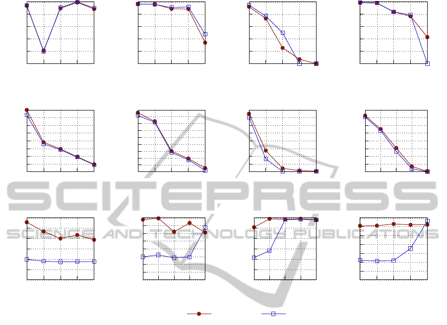
5.3 Results
The experiments are designed to compare the perfor-
mance of SIFT-EST to SIFT. Considering the exper-
imental results as shown in Figure 4, the following
trends can be observed. The precision of SIFT-EST is
almost always nearly equal to SIFT or slightly better.
This shows that the accuracy of the correspondences
is not compromised by the new matching scheme. In
case of high viewpoint changes (last samples of Graf
and Wall sets), due to the strict threshold of the initial
matching phase, no matches are found by SIFT-EST.
The respective undefined precision values (
0
0
) are re-
placed by zeros for better visualization.
Considering the number of detected matches,
SIFT-EST performs comparable to SIFT. Although
SIFT finds generally more matches than SIFT-EST,
the difference is in most cases insignificant. One rea-
son for the reduction of detected matches is the low
ratio threshold of the initial matching step, which re-
jects many correspondences that would be accepted
by SIFT. Furthermore, in cases where SIFT-EST
achieves higher precision values than SIFT, a part of
the decrease in the number of matches can be ex-
plained by the removal of some mismatches, which
is implied by the higher precision.
Regarding the processing time of the matching
phase, it can be seen that the expected improvement is
attained. There exists a noticeable separation between
SIFT and SIFT-EST in general. A reduction of order
two to three can be observed at most samples. In a
few cases, the matching time of SIFT-EST is slightly
higher than SIFT. The reason is the indistinctness of
the features, which is indicated by the low number of
matches. If the detected features are highly indistinc-
tive, a high fraction of features, or even all of them,
are checked in the initial matching step. This step has
the same computational complexity as the matching
step of SIFT. The additional costs of the SIFT-EST
method (changing the order of matching, homogra-
phy estimation, determination of relevant features) re-
sult in a matching time higher than SIFT. However,
considering the results in Figure 4 one can see that
in all these extreme cases also SIFT does not perform
well. The low number of matches found by SIFT and
their low precision makes the correspondences unus-
able for most common applications.
In these experiments, the matching step allocated
only around 7% to 13% of the overall processing
time. Therefore the achieved improvement may not
seem critical. However, it should be noticed that the
utilized images have relatively low resolutions (be-
tween 765 × 512 and 1000 × 700 pixels). In high-
resolution images, the number of detected features in-
creases drastically. Since the complexity of match-
ing is quadratic in number of features, the matching
phase seizes a higher portion of the overall computa-
tion time by increasing the resolution. Accordingly
the effect of the improvement gets more significant.
Some examples of the results of SIFT and SIFT-
EST are presented in the appendix.
6 CONCLUSION
In this paper, a SIFT-based matching algorithm was
proposed and evaluated. The aim of the method was
reducing the processing time of SIFT without com-
promising its performance. Considering the experi-
mental results, we can conclude that SIFT-EST could
fulfill these requirements. In most cases, a reduction
of order two to three could be observed in the process-
ing time of the matching step. The precision values
of SIFT-EST are nearly equal to SIFT and in some
cases even outreached it. The number of detected
matches of SIFT-EST was often lower than SIFT, but
in most cases this number would still be sufficient for
the common applications.
SIFT-EST-ASIFT-basedFeatureMatchingAlgorithmusingHomographyEstimation
509
0
20
40
60
80
100
1 2 3 4 5
Precision (%)
Image-Pair ID
BARK (Scale+Rotation)
SIFT
SIFT-EST
0
100
200
300
400
500
600
700
800
1 2 3 4 5
Matches
Image-Pair ID
BARK (Scale+Rotation)
0
0.1
0.2
0.3
0.4
0.5
0.6
1 2 3 4 5
Matching Time (s)
Image-Pair ID
BARK (Scale+Rotation)
0
20
40
60
80
100
1 2 3 4 5
Precision (%)
Image-Pair ID
BOAT (Scale+Rotation)
0
100
200
300
400
500
600
700
800
900
1 2 3 4 5
Matches
Image-Pair ID
BOAT (Scale+Rotation)
0
0.05
0.1
0.15
0.2
0.25
0.3
0.35
0.4
1 2 3 4 5
Matching Time (s)
Image-Pair ID
BOAT (Scale+Rotation)
0
20
40
60
80
100
1 2 3 4 5
Precision (%)
Image-Pair ID
GRAF (Viewpoint Change)
0
100
200
300
400
500
600
700
800
1 2 3 4 5
Matches
Image-Pair ID
GRAF (Viewpoint Change)
0
0.05
0.1
0.15
0.2
0.25
0.3
1 2 3 4 5
Matching Time (s)
Image-Pair ID
GRAF (Viewpoint Change)
0
20
40
60
80
100
1 2 3 4 5
Precision (%)
Image-Pair ID
WALL (Viewpoint Change)
0
200
400
600
800
1000
1200
1400
1600
1 2 3 4 5
Matches
Image-Pair ID
WALL (Viewpoint Change)
0
0.1
0.2
0.3
0.4
0.5
0.6
0.7
1 2 3 4 5
Matching Time (s)
Image-Pair ID
WALL (Viewpoint Change)
Figure 4: The experimental results of all four sets.
REFERENCES
Bay, H., Ess, A., Tuytelaars, T., and Van Gool, L. (2008).
Speeded-Up Robust Features (SURF). Comput. Vis.
Image Underst., 110(3):346–359.
Grauman, K. and Leibe, B. (2011). Visual Object Recogni-
tion. Synthesis Lectures on Artificial Intelligence and
Machine Learning. Morgan & Claypool Publishers.
Harris, C. and Stephens, M. (1988). A combined Corner
and Edge Detector. In In Proc. of Fourth Alvey Vision
Conference, pages 147–151.
Hartley, R. and Zisserman, A. (2004). Multiple View Geom-
etry in Computer Vision. Cambridge University Press,
ISBN: 0521540518, second edition.
Ke, Y. and Sukthankar, R. (2004). PCA-SIFT: A More Dis-
tinctive Representation for Local Image Descriptors.
In Proceedings of the 2004 IEEE Computer Society
Conference on Computer Vision and Pattern Recogni-
tion, 2004, volume 2, pages II–506–II–513 Vol.2.
Lepetit, V. and Fua, P. (2006). Keypoint Recognition using
Randomized Trees. Pattern Analysis and Machine In-
telligence, IEEE Transactions on, 28(9):1465–1479.
Lowe, D. G. (2004). Distinctive Image Features from Scale-
Invariant Keypoints. International Journal of Com-
puter Vision, 60(2):91–110.
Mikolajczyk, K. and Schmid, C. (2002). An Affine Invari-
ant Interest Point Detector. In Computer Vision-ECCV
2002, pages 128–142. Springer.
Mikolajczyk, K. and Schmid, C. (2004). Scale & Affine In-
variant Interest Point Detectors. International journal
of computer vision, 60(1):63–86.
Mikolajczyk, K. and Schmid, C. (2005). A Performance
Evaluation of Local Descriptors. Pattern Analy-
sis and Machine Intelligence, IEEE Transactions on,
27(10):1615–1630.
Mount, D. M. (1998). ANN Programming Manual. Tech-
nical report, Department of Computer Science and In-
stitute for Advanced Computer Studies, University of
Maryland.
Wu, J., Cui, Z., Sheng, V. S., Zhao, P., Su, D., and Gong, S.
(2013). A Comparative Study of SIFT and its Variants.
Measurement Science Review, 13(3):122–131.
Yu, G. and Morel, J.-M. (2011). ASIFT: An Algorithm for
Fully Affine Invariant Comparison. Image Processing
On Line, 1.
VISAPP2015-InternationalConferenceonComputerVisionTheoryandApplications
510
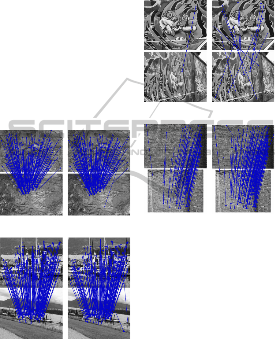
APPENDIX
For better comparison between SIFT-EST and SIFT,
some examples of the outputs of the methods are pre-
sented in this appendix. From each set, one sample
(the fourth image-pair) is chosen for the demonstra-
tion. This specific sample has been chosen due to
the moderate number of matches for almost all sets,
which allows for better illustration. The respective
matches are visualized in Figures 5 to 8.
It can clearly be seen in Figures 5, 6 and 8 that
SIFT-EST can improve the accuracy of SIFT by dis-
carding some of its mismatches. The Graf set, as
demonstrated in Figure 7, can be seen as the worst
case. Due to the strong distortion, both methods failed
in finding enough correspondences. From 14 matches
found by SIFT, only one was correct, and SIFT-EST
found a single match, which was incorrect.
(a) SIFT-EST (b) SIFT
Figure 5: Example of the results of the Bark set.
(a) SIFT-EST (b) SIFT
Figure 6: Example of the results of the Boat set.
(a) SIFT-EST (b) SIFT
Figure 7: Example of the results of the Graf set.
(a) SIFT-EST (b) SIFT
Figure 8: Example of the results of the Wall set.
SIFT-EST-ASIFT-basedFeatureMatchingAlgorithmusingHomographyEstimation
511
