
Active Perception
Improving Perception Robustness by Reasoning about Context
Andreas Hofmann
1,2
and Paul Robertson
1
1
Dynamic Object Language Labs, Inc., 114 Waltham St., Lexington, MA, U.S.A.
2
Massachusetts Institute of Technology, 77 Massachusetts Ave., Cambridge, MA, U.S.A.
Keywords:
Active Perception, POMDP, Belief State Planning.
Abstract:
Existing machine perception systems are too inflexible, and therefore cannot adapt well to environment uncer-
tainty. We address this problem through a more dynamic approach in which reasoning about context is used to
actively and effectively allocate and focus sensing and action resources. This Active Perception approach pri-
oritizes the system’s overall goals, so that perception and situation awareness are well integrated with actions
to focus all efforts on these goals in an optimal manner. We use a POMDP (Partially Observable Markov De-
cision Process) framework, but do not attempt to compute a comprehensive control policy, as this is intractible
for practical problems. Instead, we employ Belief State Planning to compute point solutions from an initial
state to a goal state set. This approach automatically generates action sequences for sensing operations that
reduce uncertainty in the belief state, and ultimately achieve the goal state set.
1 INTRODUCTION
Existing machine perception systems do not adapt
well to environmental uncertainty because their com-
ponents are statically configured to operate optimally
under very specific conditions. As a result, informa-
tion flow in such systems is bottom up, and generally
not guided by knowledge of higher level context and
goals.
If higher level goals, context, or the environment
change, the specific conditions for which the static
configuration is intended may no longer hold. As a
result, the static systems are prone to error because
they cannot adapt to the new conditions. In addition
to their inflexibility, existing machine perception sys-
tems are often not well integrated into the autonomous
and systems to which they provide information. As
a result, they are unaware of the autonomous sys-
tem’s overall goals, and therefore, cannot make intel-
ligent observation prioritization decisions in support
of these goals.
We address these shortcomings by using a more
dynamic approach in which reasoning about context
is used to actively and effectively allocate sensing re-
sources. This Active Perception approach prioritizes
the system’s overall goals, so that perception and situ-
ation awareness are well integrated with actions to fo-
cus all efforts on these goals. Active perception draws
on models to inform context-dependent tuning of sen-
sors, to direct sensors towards phenomena of greatest
interest, to follow up initial alerts from cheap, inac-
curate sensors with targeted use of expensive, accu-
rate sensors, and to intelligently combine results from
sensors with context information (gists) to produce in-
creasingly accurate results.
Consider the problem of changing a flat tire on a
car. This has been a “textbook” problem for PDDL
generative planning systems (Fourman, 2000), and
also a challenge problem in the Defense Advanced
Research Project Agency (DARPA) ARM project
(Hebert et al., 2012). There are significant challenges
in building an autonomous system that can perform
this task entirely, or even one that would just assist
with the task (Figure 1). Such a system would have
to be able to determine the vehicle type (Figure 2),
whether a tire is actually flat (Figure 3), and what an
appropriate sequence of repair steps should be (Figure
4). It would have to be able to solve many subprob-
lems, such as reliably finding a wheel in an image.
The system would have to be able to work in many
different environments, a great range of lighting con-
ditions, and for a comprehensive set of vehicle types.
We consider the sub-problem of reliably finding
the wheels of a vehicle in an image. We show how
the use of top-down, model-based reasoning can be
used to coordinate the efforts of multiple perception
328
Hofmann A. and Robertson P..
Active Perception - Improving Perception Robustness by Reasoning about Context.
DOI: 10.5220/0005298103280336
In Proceedings of the 10th International Conference on Computer Vision Theory and Applications (VISAPP-2015), pages 328-336
ISBN: 978-989-758-090-1
Copyright
c
2015 SCITEPRESS (Science and Technology Publications, Lda.)

(a) Fully autonomous sys-
tem using robot.
(b) Semi-autonomous advi-
sory system.
Figure 1: Intelligent machine perception would be needed
for both a fully autonomous system (a), and a semi-
autonomous advisory system (b). The latter might include
observation drones, and Google glasses (Bilton, 2012) to
guide a human user in the repair.
(a) Truck (b) SUV (c) Sedan
Figure 2: Vehicle type, and ultimately, make and model,
are useful things for the perception system to know (or to
discover).
(a) Tire is flat. (b) Tire is under-
inflated.
(c) Tire is OK.
Figure 3: The perception system must be able to determine
whether a tire is really flat, and which one it is.
(a) Wheel chock. (b) Remove wheel.
Figure 4: Repair steps include stabilizing the car (a), getting
the spare tire and tools, jacking up the car, removing lug
nuts and wheel (b), and installing the new wheel.
algorithms, resulting in more robust, accurate perfor-
mance than is achievable through use of individual al-
gorithms operating in a bottom-up way.
2 PROBLEM STATEMENT
Given one or more agents operating in an environ-
ment, and given that the agents do not directly know
the state of the environment, or even, possibly, parts
of their own state, and given a goal state for the en-
vironment and agents, the problem to be solved is to
compute control actions for the agents such that the
goal is achieved. In this case, an agent is a resource
capable of changing the environment (and its own)
state, by taking action. An agent could be a mobile
ground robot, a sensing device, or one of many par-
allel vision processing algorithms running on a clus-
ter, for example. Given that there is uncertainty in
the state, an agent must estimate it based on (possibly
noisy) observations. Based on the agent’s best esti-
mate of the current state, it should take actions that
affect the state in a beneficial way.
The actions, themselves have some uncertainty;
they do not always achieve the intended effect on the
state. The agents must take both state estimate un-
certainty, and action uncertainty into account when
determining the best course of action. Actions can
also have cost. The agents must balance the cost of
actions against the reward of reduced uncertainty and
progress towards the goal when deciding on actions.
This problem presents significant challenges.
First, the overall state space can be very large. Sec-
ond, the state space is generally hybrid; it includes
discrete variables, such as hypotheses for vehicle
type, as well as continuous variables, such as posi-
tion of a wheel. Third, significant parts of the state
space may not be directly measurable, and must be
estimated based on observations. Fourth, the effect of
some actions on state may have uncertainty. Fifth, the
agents must take many considerations into account
when deciding on actions: they must take into account
the uncertainty of the state estimate, the uncertainty
of the action effect on the state, the cost of the ac-
tion, and the benefit of the action in terms of reducing
uncertainty and making progress towards the goal.
Note that some actions are performed to im-
prove situational awareness, and some actions are per-
formed to change the state of the agent and/or en-
vironment, to achieve an overall goal (for example,
jacking up a car so the tire can be changed). The au-
tonomous system should judiciously mix both types
of actions so that the situational awareness is suffi-
cient to achieve the goal. In particular, a good se-
quence of control actions is one that minimizes cost,
where cost attributes include both state uncertainty, as
well as cost of the action itself. Note, also, that it is
typically not necessary for the system to exhaustively
resolve all state uncertainty; it just needs to be certain
enough to achieve the overall goal.
The problem is stated formally as follows. Let
S =
{
S
e
, S
a
}
be the state space, where S
e
is for the
environment, and S
a
is for the agent; let A be the set
of agent actions, and O, the set of observations. A
ActivePerception-ImprovingPerceptionRobustnessbyReasoningaboutContext
329

state transition model represents state evolution prob-
abilistically as a function of current state and action:
T : S × A × S 7→ [0, 1]. An observation model rep-
resents likelihood of an observation as a function of
action and current state: Ω : O × A × S 7→ [0, 1]. A
reward model represents reward associated with state
evolution: R : S × A × S 7→ R. Given an initial state s
0
and goal states s
g
, the problem to be solved is to com-
pute an action sequence a
0
, . . . a
n
such that s
n
∈ s
g
,
and R is maximized. Note that this problem formu-
lation, expressed in terms of a single agent, is easily
extended to allow for multiple agents.
3 BACKGROUND AND RELATED
WORK
A Partially Observable Markov Decision Process
(POMDP) (Monahan, 1982) is a useful framework for
formulating problems for autonomous systems where
there is uncertainty both in the sensing and actions. A
POMDP is a tuple
h
S, A, O, T, R, Ω, γ
i
where S is a (fi-
nite, discrete) set of states, A is a (finite) set of actions,
O is a (finite) set of observations, T : S×A×S 7→ [0, 1]
is the transition model, R : S × A × S 7→ R is the re-
ward function associated with the transition function,
Ω : O ×A×S 7→ [0, 1] is the observation model , and γ
is the discount factor on the reward. The belief state is
a probability distribution over the state variables, and
is updated each control time increment using recur-
sive predictor/corrector equations. First, the a priori
belief state (prediction) for the next time increment,
¯
b(s
k+1
), is based on the a posteriori belief state for
current time increment.
¯
b(s
k+1
) =
∑
s
k
Pr (s
k+1
|s
k
, a
k
)
ˆ
b(s
k
)
=
∑
s
k
T (s
k
, a
k
, s
k+1
)
ˆ
b(s
k
)
(1)
Next, the a posteriori belief state (correction) for the
next time increment,
ˆ
b(s
k+1
), is based on the a priori
belief state for next time increment.
ˆ
b(s
k+1
) = α Pr (o
k+1
|s
k+1
)
¯
b(s
k+1
)
= α Ω(o
k+1
, s
k+1
)
¯
b(s
k+1
)
(2)
α =
1
Pr (o
k+1
|o
1:k
, a
1:k
)
(3)
These equations work well given that the models
are known, and given that the control policy for select-
ing an action based on current belief state is known.
Unfortunately, computing these, particularly the con-
trol policy, is a challenging problem. Value iteration
(Zhang and Zhang, 2011) is a technique that computes
a comprehensive control policy, but it only works for
very small problems. An alternative is to abandon
computation of a comprehensive control policy, and
instead, compute point solutions for a particular ini-
tial state and goal state set.
A promising technique for this is Belief State
Planning (Kaelbling and Lozano-P
´
erez, 2013), which
is based on generative planner technology (Helmert,
2006). A key idea in this technique is the use of two
basic actions for a robotic agent: move and look. A
move action changes the state of the robot and/or en-
vironment; it may move the robot in the environment,
for example. A look action is intended to improve the
robot’s situational awareness.
The move action is specified using a PDDL-like
description language.
Move(lstart, ltarget)
effect: BLoc(ltarget, eps)
precondition: BLoc(lstart, moveRegress(eps))
cost: 1
The variables lstart and ltarget denote the initial
and final locations of the robot. The effect clause
specifies conditions that will result from performing
this operation, if the conditions in the precondition
clause are true before it is executed. Cost of the
action is specified in the cost clause. The function
BLoc(loc, eps) returns the belief that the robot is at
location loc with probability at least (1 - eps). The
moveRegress function determines the minimum con-
fidence required in the location of the robot on the
previous step, in order to guarantee confidence eps in
its location at the resulting step:
moveRegress(eps) =
eps − p
f ail
1 − p
f ail
(4)
where p
f ail
is the probability that the move action will
fail.
The look action is specified as follows:
Look(ltarget)
effect: BLoc(ltarget, eps)
precondition: BLoc(lstart,
lookPosRegress(eps))
cost: 1 - log(posObsProb
(lookPosRegress(eps)))
The lookPosRegress function takes a value eps
and returns a value eps’ such that, if the robot is be-
lieved with probability at least 1 eps’ to be in the tar-
get location before a look operation is executed and
the operation is successful in detecting ltarget, then it
will be believed to be in that location with probability
at least 1 eps afterwards.
lookPosRegress(eps) =
eps(1 − p
f n
)
eps(1 − p
f n
) + p
f p
(1 −eps)
(5)
VISAPP2015-InternationalConferenceonComputerVisionTheoryandApplications
330
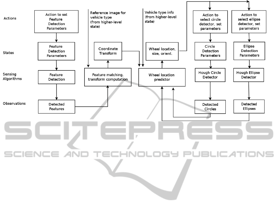
Figure 5: Data flow architecture for wheel finding components.
where p
f n
and p
f p
are the false negative and false
positive observation probabilities.
In terms of the POMDP belief state update, the
move action corresponds to the predictor (Eq. 1), and
the look action corresponds to the corrector (Eq. 2).
For the observations, we make extensive use of
two types of feature detection algorithms: Speeded
Up Robust Features (SURF) (Bay et al., 2008), and
Hough Transforms (Duda and Hart, 1972). Neither of
these algorithms, used individually, is satisfactory for
solving the wheel detection problem robustly. How-
ever, when used together, in an Active Perception
framework, they beneficially reinforce each others’
hypotheses, allowing for more reliable performance.
4 APPROACH
When evaluating approaches to this problem, it is use-
ful to consider what an architecture for the sensors
and state estimation components should look like if
it were designed by a human expert (Figure 5). Each
sensing algorithm can use the current belief state as
input, and can also adjust belief state as output.
This organization based on actions, observations,
and belief state fits well with the POMDP formal-
ism. As stated previously, we avoid value iteration ap-
proaches (Zhang and Zhang, 2011), and instead com-
pute point solutions. Our approach automatically syn-
thesizes architectures such as the one in Figure 5, and
generates action sequences for sensing operations that
reduce uncertainty in the belief state, and ultimately
achieve the goal state set.
We use three main sensing actions: SURF Match,
SURF Match Other Wheel, and Hough Ellipse Match.
Each of these actions has preconditions (requirements
for current belief state), and post conditions (effects
on belief state). SURF Match uses the SURF algo-
rithm to perform a preliminary detection of a wheel
in an image. SURF Match Other Wheel attempts to
find the second wheel, also using SURF, given that
the first wheel has been detected. This action also
performs vehicle pose estimation, and refines the pre-
diction of where the wheels are. Hough Ellipse Match
uses either a Hough Circle or Hough Ellipse trans-
form algorithm to refine the wheel location estimates.
The sequence of actions is computed using a gen-
erative planner. Given the high uncertainty in our
problem, the traditional approach of generating a plan
and executing it in its entirety is not suitable. Instead,
we adopt a receding horizon control framework in
which a plan is generated based on the current belief
state, but only the first action of this plan is executed.
After the action, the belief state is updated based on
observations, and an entirely new plan is generated.
The process then repeats with the first action from this
new plan being executed. This approach is computa-
tionally intensive, but it ensures that all actions are
based on the most current belief state.
To implement this receding horizon control frame-
work, we use an architecture consisting of four main
components: Executive, Planner, Sensor Actions, and
Belief State Updater, as shown in Figure 6. The Ex-
ecutive manages the receding horizon control process.
It maintains the current belief state, and the goal state
set. At each control loop iteration, it passes these to
the Planner. The Planner, if successful, returns a plan
consisting of actions that transition the system from
the current state to a goal state, if there are no distur-
ActivePerception-ImprovingPerceptionRobustnessbyReasoningaboutContext
331
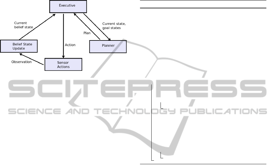
bances. The Executive takes the first action from the
plan and executes it by dispatching the appropriate
sensor operation. The sensor operation produces an
observation, which is used to update the belief state.
The process then repeats.
Figure 6: Receding Horizon Control Architecture for Active
Perception.
5 IMPLEMENTATION
The Executive component implements the top-level
receding horizon control loop, coordinating the activi-
ties of the planner and sensor components. Algorithm
1 shows pseudocode for the Executive. The algorithm
begins by initializing the belief state according to the
a priori probabilities, and performing other initializa-
tion (Line 1). Belief state for a discrete state vari-
able is represented as a Probability Mass Function
(PMF) over the possible values of the probabilistic
variable. Belief state for a continuous state variable is
represented using a Gaussian Probability Distribution
Function (Gaussian PDF) with a specified mean and
variance. This could be extended to a representation
using a mixture of Gaussians, in order to approximate
more complex, non-Gaussian PDFs.
The receding horizon control loop begins at Line
5. The first step is to invoke the generative planner
in order to determine the next action. A generative
planner requires, as one of its inputs, the current state
in a deterministic form. The belief state, however,
is represented in a probabilistic form, so it first has
to be converted to a deterministic form using Most-
LikelyState (Line 6). The input to the generative plan-
ner includes the determinized state, as well as the goal
state set. The Executive generates domain and prob-
lem PDDL files, and then executes the planner (Line
7). The planner generates a result file containing a
plan, which the Executive reads.
The planner may fail to generate a plan, in which
case, the algorithm returns failure. If the planner
is successful in generating a plan, the executive dis-
patches the first action (Line 11). The action (sensor
operation) generates an observation. The belief state
is updated based on this observation (Line 12). The
algorithm terminates if the goal has been achieved,
or the maximum number of iterations has been ex-
ceeded.
Algorithm 1: Executive.
Input: a-priori-belief-state-probabilities, goal-state-set
Output: goal-achieved?
/* Perform initialization. */
1 belief-state ←
InitializeBeliefState(a-priori-belief-state-probabilities);
2 goal-achieved? ← f alse;
3 max-iterations ← 1000;
4 iteration ← 0;
/* Begin control loop. */
5 while not goal-achieved? do
6 current-state ← MostLikelyState(belief-state);
7 plan? ← GeneratePlan(current-state, goal-state-set);
8 if not plan? then
9 return ;
10 action ← First(plan?);
11 observation ← Dispatch(action);
12 belief-state ← UpdateBeliefState(observation);
13 goal-achieved?
← CheckGoalAchieved(belief-state, goal-state-set);
14 iteration ← iteration + 1;
15 if iteration > max-iterations then
16 return ;
The Planner component is implemented using
Fast Downward (Helmert, 2006), a state of the art
generative planner that accepts problems formulated
in the PDDL language (McDermott et al., 1998). A
PDDL problem formulation consists of a domain file,
and a problem file. The domain file specifies types
of actions that can be used across a domain of appli-
cation such as logistics, manufacturing assembly, or
in this case, finding wheels in an image. The domain
file is fixed; it does not change for different problems
within the domain. Thus, this part of the formulation
was generated manually, and is not modified by the
Executive. The problem file, on the other hand, con-
tains problem-specific information such as initial and
goal states. Therefore, it must be generated specifi-
cally for any new problem. The Executive generates
this file automatically, based on knowledge of the goal
and belief states. The following PDDL domain file
fragment shows the definition of the SURF Match ac-
tion in PDDL.
(:action SURF-match
:parameters
(?w ?p ?bsv)
:precondition
VISAPP2015-InternationalConferenceonComputerVisionTheoryandApplications
332

(and (belief-state-variable ?bsv)
(pose ?p) (wheel ?w)
(for-wheel ?w ?bsv)
(at-pose ?p ?bsv)
(at-belief-level
belief-level-one ?bsv))
:effect
(and (at-belief-level
belief-level-two ?bsv)
(increase
(total-cost)
(feature-observation-cost ?p))))
The precondition clause specifies that the belief state
variable value for a particular pose and wheel must
be at belief level one in order for this operation to
be tried. The effect clause specifies that the belief
level increases to belief-level-two if the operation suc-
ceeds. The cost for the operation is also added to the
total cost. The other sensor actions are specified in
the PDDL domain file in a similar manner.
We now describe in more detail the three sensor
actions: SURF Match, SURF Match Other Wheel,
and Hough Ellipse Match. The SURF Match ac-
tion uses the SURF (Speeded Up Robust Features)
algorithm (Bay et al., 2008) to attempt to identify
wheels by matching a wheel in a reference image with
a wheel in the target image. The SURF algorithm
is scale invariant, but is somewhat sensitive to large
changes in orientation. Therefore, multiple reference
images are used, including ones for different orien-
tations (Figure 7). The orientations in the reference
images correspond to the orientations of the discrete
belief state variables.
(a)
+2
(b) +1 (c) 0 (d) -1 (e) -2
Figure 7: Wheel reference images, corresponding to differ-
ent orientations.
The SURF Match action is not highly reliable; it
can miss detecting a wheel, especially if the target im-
age is noisy, and it can falsely detect objects that are
not wheels. Also, due to the symmetry of wheel im-
ages, the SURF Match algorithm does not provide a
very accurate estimate of the pose (position and ori-
entation) of the wheel in the target image. Thus, the
SURF Match action is used to attempt to achieve a
rough initial match, the goal being to move from low
to medium confidence estimates, and set the stage for
the use of the other sensor actions to improve the es-
timates.
The SURF Match Other Wheel sensor action is
similar to the SURF Match action, but assumes that
one wheel position estimate already exists. It uses this
information, along with a number of gists (assump-
tions), to try to find the other wheel. In particular, it
is assumed that the action is observing the left side of
the car, and that the car is on level terrain.
If the SURF Match Other Wheel action is success-
ful in finding the other wheel, then it uses the posi-
tion estimates of both wheels to estimate the pose of
the car. The sensor action uses projective geometry,
combined with a number of additional gists, to esti-
mate the positions of each wheel in the world coordi-
nate frame, given the image position estimates. These
gists are: 1) the height of the camera; 2) the focal
length of the camera; and 3) the size of the wheel. All
of these are reasonable gists; a ground robot or UAV
would know the focal length of its camera, as well as
its height. Given previous gists for vehicle type, the
size of the wheel can be determined from the vehicle
type’s spec data.
Once the position estimates of each wheel in the
world coordinate frame are known, simple trigonom-
etry is used to determine orientation of the car, partic-
ularly, its yaw (rotation about the vertical axis). This
estimate is the continuous counterpart to the discrete
belief state variables for orientation. The continuous
and discrete variables inform and reinforce each other
as part of the belief state update mechanism.
The Hough Ellipse Match sensor action uses
Hough transforms (Duda and Hart, 1972) to deter-
mine wheel position in an image with a high degree
of accuracy. This action is computationally expen-
sive, but has the potential to give very accurate esti-
mates, when supplied with good parameters. Thus,
this action is used after the other, less expensive sen-
sor actions have developed a good hypothesis about
the wheel pose.
The computational expense of the Hough trans-
form algorithm rises as the number of parameters in-
creases. Therefore, the ellipse variant is more expen-
sive than the circle variant. For this reason, the Hough
Ellipse Match sensor action first checks whether esti-
mated orientation (yaw angle) of the car is small, indi-
cating that the car side is facing the camera directlym
ub wgucg case the circle variant is used.
ActivePerception-ImprovingPerceptionRobustnessbyReasoningaboutContext
333
6 RESULTS AND DISCUSSION
6.1 Negative Results using Individual
Sensor Algorithms
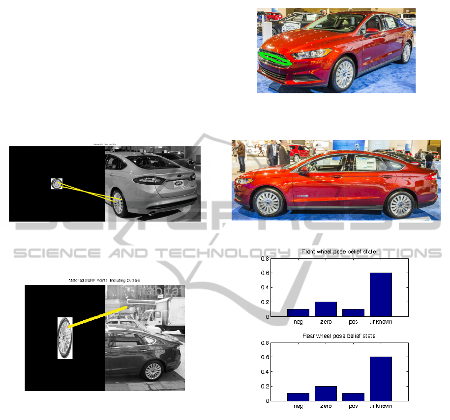
The SURF algorithm is susceptible to error, particu-
larly when there is a significant difference in orien-
tation between the wheel in the reference and target
images. Figure 8 shows a weak match result due to
this problem. Figure 9 shows an incorrect match, also
due to this problem.
Figure 8: The significant difference in wheel orientation be-
tween the reference and target images results in a match of
only two points. This does not give a very good estimate of
wheel position.
Figure 9: The significant difference in wheel orientation be-
tween the reference and target images results in a bad match
(false positive).
For this reason, our system uses multiple wheel
reference images, at different orientations. Which to
use is informed by the belief state variables.
Figure 10 shows what can easily happen when
the Hough Ellipse algorithm is used with insufficient
guidance. Instead of finding a wheel, the algorithm
has found an elliptical form in the car’s grill. Suf-
ficiently constraining the expected ellipse parameters
solves this problem.
6.2 Example Test Cases
For the first test case, the target image is as shown
in Figure 11. The a priori belief state for the discrete
wheel poses is shown in Figure 12 (values for car pose
belief state are similar). This indicates that the poses
Figure 10: With insufficient guidance, the Hough algo-
rithm finds an ellipse in the car’s grill (highlighted in green),
rather than finding the wheel.
Figure 11: Target image for test case 1.
(a) Wheel
Figure 12: Wheel pose, a priori belief state.
are largely unknown, with a slight bias to the zero
pose.
The first control step iteration, based on this be-
lief state, yields the following plan from the PDDL
planner.
1. SURFMatch(front-wheel pose-zero)
2. SURFMatchOtherWheel(front-wheel pose-zero)
3. HoughEllipseMatch(rear-wheel pose-zero)
The Executive performs the first of these actions,
yielding a successful match, as shown in Figure 13.
Based on this, wheel pose estimates are updated;
the hypothesis for zero pose for the front wheel is
strengthened.
The second control step iteration, based on this
VISAPP2015-InternationalConferenceonComputerVisionTheoryandApplications
334
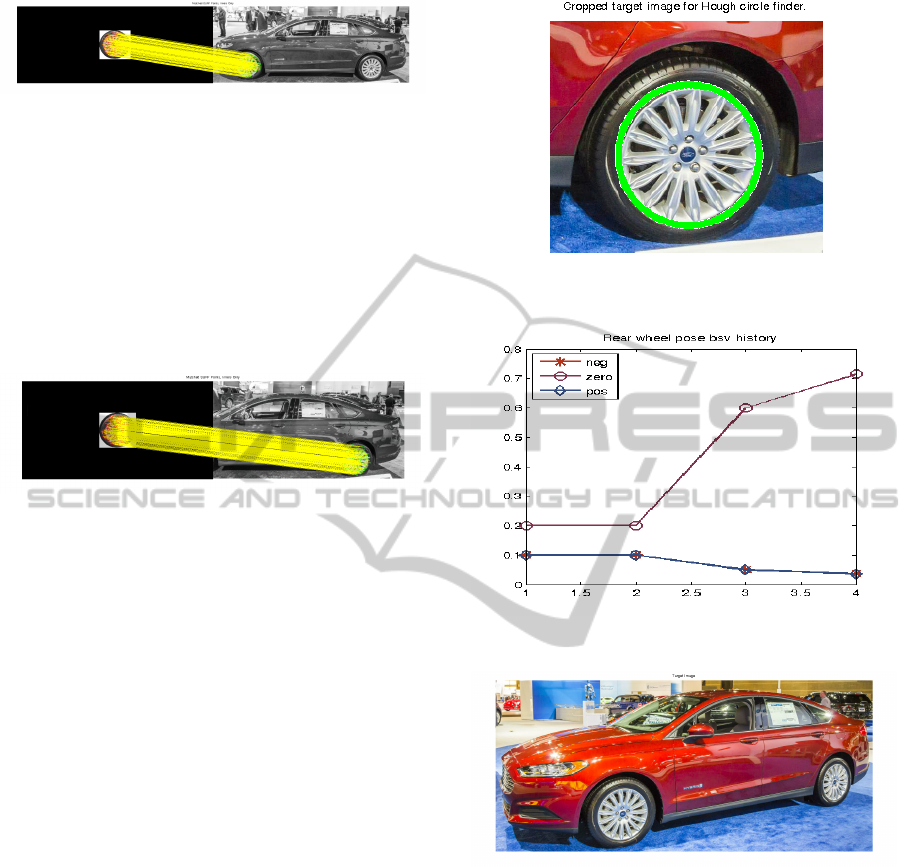
Figure 13: Successful SURF match to front wheel.
updated belief state, yields the following plan from
the PDDL planner.
1. SURFMatchOtherWheel(front-wheel pose-zero)
2. HoughEllipseMatch(rear-wheel pose-zero)
The Executive performs the first of these actions,
yielding a successful match, as shown in Figure 14.
Based on this, wheel and car pose estimates are up-
dated to further strengthen the zero pose hypothesis.
Figure 14: Successful SURF match to other (rear) wheel.
The third control step iteration, based on this up-
dated belief state, yields the following plan from the
PDDL planner.
1. HoughEllipseMatch(rear-wheel pose-zero)
The Executive performs the first of these actions,
yielding a successful match, as shown in Figure 15. In
this case, because the pose hypothesis is pose zero (in-
dicating that the camera is directly facing the car), the
circle rather than ellipse variant of the Hough trans-
form is used. The history of rear wheel pose belief
state values over the control iterations is shown in
Figure 16. The zero pose belief increases with suc-
cessive iterations (observations), whereas the pos and
neg pose beliefs decrease.
For second test case, the target image is as shown
in Figure 17. As before, the planner generates a plan
assuming pose zero, based on the a priori belief state.
The SURF matches succeed, even though the refer-
ence image for pose zero does not exactly match the
wheels in the car due to its angle. After the SURF
match other wheel action, the pose estimate is im-
proved, resulting in a belief state where pose -1 is
most likely. The Hough ellipse match action knows
that with this pose, the circle variation of the algo-
rithm will not work, so it uses the ellipse variation,
with bounds on aspect ratio and rotation informed by
the car pose estimate. This results in a successful
match, as shown in Figure 18. The history of rear
wheel pose belief state values over the control itera-
tions is shown in Figure 19. The zero pose belief is
Figure 15: Successful Hough ellipse match to rear wheel
(match highlighted in green).
Figure 16: Evolution of belief state for rear wheel pose vari-
able (neg, zero, and pos values).
Figure 17: Target image for test case 2.
initally the highest, but after the SURF match other
wheel action (iteration 2), it drops, along with the pos
pose belief, while the neg pose belief increases.
The focus of our efforts thus far has been on the
sub-problem of finding a wheel in an image. This has
led to an emphasis on “look” actions, but no incorpo-
ration of “move” actions (actions that change the state
of the environment). We believe that the approach we
have developed is well suited for incorporating move
as well as look actions, with the generative planning
component intelligently combining both types of ac-
tions. This would allow for testing with more general
kinds of problems, where the goal is more than purely
a perception goal, but rather, involves achieving an
environment goal.
ActivePerception-ImprovingPerceptionRobustnessbyReasoningaboutContext
335
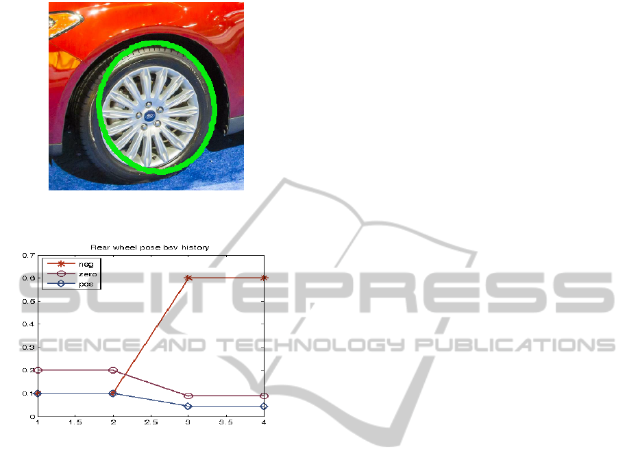
Figure 18: Successful Hough ellipse match, using ellipse
rather than circle variation of the algorithm.
Figure 19: Evolution of belief state for rear wheel pose vari-
able, example test case 2.
ACKNOWLEDGEMENTS
This research was developed with funding from
DARPA. The views, opinions, and/or findings con-
tained in this article are those of the authors and
should not be interpreted as representing the official
views or policies of the Department of Defense or the
U.S. Government.
REFERENCES
Bay, H., Ess, A., Tuytelaars, T., and Van Gool, L. (2008).
Speeded-up robust features (surf). Computer vision
and image understanding, 110(3):346–359.
Bilton, N. (2012). Behind the google goggles, virtual real-
ity. New York Times, 22.
Duda, R. O. and Hart, P. E. (1972). Use of the hough trans-
formation to detect lines and curves in pictures. Com-
munications of the ACM, 15(1):11–15.
Fourman, M. P. (2000). Propositional planning. In Pro-
ceedings of AIPS-00 Workshop on Model-Theoretic
Approaches to Planning, pages 10–17.
Hebert, P., Hudson, N., Ma, J., Howard, T., Fuchs, T.,
Bajracharya, M., and Burdick, J. (2012). Combined
shape, appearance and silhouette for simultaneous
manipulator and object tracking. In Robotics and Au-
tomation (ICRA), 2012 IEEE International Confer-
ence on, pages 2405–2412. IEEE.
Helmert, M. (2006). The fast downward planning system.
J. Artif. Intell. Res.(JAIR), 26:191–246.
Kaelbling, L. P. and Lozano-P
´
erez, T. (2013). Inte-
grated task and motion planning in belief space.
The International Journal of Robotics Research, page
0278364913484072.
McDermott, D., Ghallab, M., Howe, A., Knoblock, C.,
Ram, A., Veloso, M., Weld, D., and Wilkins, D.
(1998). Pddl-the planning domain definition language.
Monahan, G. E. (1982). State of the arta survey of partially
observable markov decision processes: Theory, mod-
els, and algorithms. Management Science, 28(1):1–
16.
Zhang, N. L. and Zhang, W. (2011). Speeding up the
convergence of value iteration in partially observ-
able markov decision processes. arXiv preprint
arXiv:1106.0251.
VISAPP2015-InternationalConferenceonComputerVisionTheoryandApplications
336
