Localization of Visual Codes using Fuzzy Inference System

eter Bodn

ar and L

aszl

o G. Ny

Department of Image Processing and Computer Graphics, University of Szeged, Szeged, Hungary

Keywords:

QR Code, Object Detection, Pattern Recognition, Image Texture Analysis, Histogram.

Abstract:

Usage of computer-readable visual codes is common in everyday life. The reading process of visual codes

consists of two steps, localization and data decoding. This paper introduces a fast and robust method for

localization of visual codes using Fuzzy Inference Systems based on simplistic, attentive features which can

be optionally extended with cell histograms. Input image properties, assigned membership functions and

efﬁciency of the system has been evaluated and discussed, showing FIS is a viable alternative for rapid QR

code recognition in the image domain. The basic approach can be also used with lookup tables, that speeds up

image cell evaluation and makes it ideal for embedded systems.

1 INTRODUCTION

Two-dimensional visual code formats are designed

aiming automatic readability by computers and em-

bedded systems. Image quality and acquisition tech-

niques vary considerably and each application has its

own requirements for detection speed and accuracy,

making the task more complex.

The recognition process consists of two steps, lo-

calization and decoding. There already are works

proposing various ways to automatically localize

codes in images. A paper suggests localization of the

locator patterns of QR codes using three scan-lines

(Chu et al., 2011), however, this is sensitive to noise

and camera shaking. Other works (Ohbuchi et al.,

2004; Lin and Lin, 2013) involve mathematical mor-

phology, which is very tolerant to noise and blur, but

it can also be time-consuming, thus making real-time

implementations more difﬁcult on embedded systems.

There is also a work using Haar-based classiﬁer for

the locator patterns of QR codes (Belussi and Hirata,

2011), which is fast and can have high precision with

a well-chosen application setup and training database.

A QR code is attentive, which means it requires

little human observation to identify. Since its fea-

tures are observable on a higher level than the texture

of its carrier material, they are easy to recognize by

humans, but difﬁcult to quantitatively deﬁne. Terms

and operators of fuzzy logic are a viable option for

QR code localization based on statements that include

vagueness and uncertainty.

In this paper, we propose a Fuzzy Inference Sys-

tem (FIS) based on the most simplistic, attentive fea-

tures of a QR coded, and test the proposed algorithm

on other popular 2D code types. The described ap-

proach can be efﬁcient with respect to computation

time and storage, and most of the computed features

can be approximated using only a subset of pixels,

that allows ﬁne-tuning of the application to be faster

or more accurate. These properties can make FIS-

based localization a preferred choice over other ex-

isting algorithms. After the code is located, there are

reliable methods for correction of camera shaking and

orientation (Chu et al., 2011), and correction of per-

spective distortion (Ohbuchi et al., 2004). Decoding

is not discussed here, since after a successful localiza-

tion step, retrieving the embedded data can be consid-

ered straightforward.

2 THE PROPOSED

LOCALIZATION METHOD

Input image is uniformly divided into square blocks of

equal size. Each block serves as an input to the FIS.

Features are computed, and the FIS shows how likely

a QR code part is present in the block. After all blocks

are evaluated, a feature matrix is formed by the values

given for each block (Fig. 1(b)). Finally, the matrix is

evaluated and regions of interests are formed, that can

be re-mapped to image space, thus giving bounding

boxes to QR code candidates.

345

Bodnar P. and Nyúl L..

Localization of Visual Codes using Fuzzy Inference System.

DOI: 10.5220/0005299103450352

In Proceedings of the 10th International Conference on Computer Vision Theory and Applications (VISAPP-2015), pages 345-352

ISBN: 978-989-758-090-1

 2015 SCITEPRESS (Science and Technology Publications, Lda.)

(a) (b)

Figure 1: Printed QR code on tablecloth (a) and its FIS fea-

ture image (b).

2.1 The Fuzzy Inference System

The proposed FIS consists of three input and one out-

put variables. Membership function (MF) parameters

are tuned each time to the end-user scenario using

statistics of a few input images. For the selection of

properties, we pursued simple features that represent

humanly observable properties. The three properties

can be summarized in the following statement: QR

code parts consist of mostly black and white pixels of

similar amounts, while having moderate to high con-

trast and low saturation.

2.1.1 Variables and Membership Functions

Our ﬁrst variable is based on the absolute difference

of pixels from the 50 % gray value. Intensity values

referred in this paper, are normalized to [0,1] from

the 8-bit grayscale input images to ﬁt the ranges of

the membership functions. The ﬁrst property is

graydist avg =

∑

p∈block

|V (p) − 0.5| (1)

where n denotes the number of sampled pixels from

the block, and V (p) is the V value of the pixel in

HSV color space. From a couple of sample images,

blocks being fully covered with QR code parts as pos-

itive samples, and blocks with 0 % coverage ratio as

negatives, are extracted. After that, mean and stan-

dard deviation are computed for graydist avg. This

was 0.41 ± 0.04 for positive samples and 0.31 ± 0.12

for negatives in our ﬁrst test set. That would deﬁne

two Gaussian membership functions, perfect(m =

0.41,σ = 0.04) and low(m = 0.31, σ = 0.12), how-

ever, using those would let very small tolerance and

they would not cover the whole input range. To over-

come this, Z-shaped and S-shaped membership func-

tions are used instead of Gaussians (Fig. 2(a)). A rea-

sonable Z-term for low is ZMF(0,0.41), because the

mean of graydist avg was at 0.41. For perfect, an

S-term of SMF(0.31, 0.41) is proposed, since nega-

tive sample mean was 0.31, which means, from that

point, we have no information about the block con-

tent according to this property. The endpoint of the

S-term should be 0.41, since that was our measured

mean value for the test images. This parameter would

(a) (b) (c)

Figure 2: FIS input variables. (a): Mean brightness abso-

lute difference from gray: low (yellow) and perfect (red);

(b): Mean brightness: low (yellow), perfect (orange) and

high (red); (c): Mean saturation: high (red). Parameters are

indicated in the text.

be 0.5 in the perfect case, and lower values reﬂect the

amount of blurring present in blocks containing QR

code parts.

The second input variable is blockavg, the mean

intensity of the block. We obtained 0.52 ± 0.13 for

positive, and 0.44± 0.31 for negative examples. Hav-

ing this value around 0.5 for positive samples is ex-

pected because of the structure of the QR code. For

negative samples, it is dependent on the content of

the block. This property seems to have small classi-

ﬁcation power, however, having the value around 0.5

is a necessary condition for a positive sample. Three

membership functions are proposed, one Gaussian for

perfect(m = 0.52, σ = 0.13) values, a ZMF(0, 0.5)

and a SMF(0.5,1) for low and high blocks, respec-

tively (Fig. 2(b)). Both of the last two MFs express

low certainty of presence of a QR code part within

the block.

The third input parameter saturation excludes re-

gions that have high saturation, since highly saturated

areas are less likely to contain QR codes. The goal

with saturation was to improve precision while keep-

ing the hit rate. Mean saturation was 0.13 ± 0.05

for positive, and 0.39 ± 0.22 for negative samples,

so a ZMF(0.13,0.39) is proposed as high, shown in

Fig. 2(c).

The output of the FIS is codeness, the certainty

of QR code texture within a block, which can be ex-

pressed by two MFs, ZMF(0,1 − x) and SMF(x,1)

with x ∈ [0, 0.5], providing different level of smooth

transitions. We used an intermediate x = 0.33 value

in our model, thus producing ZMF(0,0.67) and

SMF(0.33,1) for low and high MFs, respecively.

2.1.2 Rules

The rule set of the FIS contains the following rules:

R1 if blockavg is perfect and graydist avg is

perfect then codeness is high

R2 if blockavg is low or blockavg is high then

codeness is low

R3 if graydist avg is low then codeness is low

R4 if saturation is high then codeness is low

VISAPP2015-InternationalConferenceonComputerVisionTheoryandApplications

346

R1 is about positive response. Having the block-

avg and graydist avg properties in range are re-

quired conditions that have to be met simultaneously.

The blockavg is needed so high codeness cannot be

achieved with solid black or solid white blocks which

both have low saturation and high graydist avg. Fol-

lowing the same logic, we assume some contrast

within blocks, expressed by graydist avg, so solid

gray blocks will not result in high codeness. R2 is

to connect low and high MFs of blockavg, since both

indicate QR code part is not likely in that block. R3

ﬁlters out blocks by graydist avg in a similar manner

than the previous one. R4 is another exclusion ﬁlter,

which is based on the mean of saturation, as discussed

above.

2.1.3 Operators

For conjunction, minimum and a couple of product

operators are available, which behave similarly, and

show no signiﬁcant difference in our case. Minimum

operator is the simplest to compute. Both blockavg

and graydist avg has to be high for high codeness,

and the decision based on the minimum of these vari-

ables suits our model. Products, like algebraic prod-

uct can also be used, however, they lead to a stricter

rule and steeper decision surface. For disjunction op-

erator, the maximum is recommended with this rule

set and MF layout, since that is the simplest operator

to compute, and in this case, where no overlapping is

present between the MFs participating in the conjunc-

tion (Fig. 2), there is no difference in the results of

maximum and the various x-sum operators available.

For the case of simplicity, minimum can be used for

activation. The usage of algebraic product would re-

sult in smoother transitions with the defuzziﬁed out-

put variable, however, it does not affect accuracy of

the FIS signiﬁcantly. For accumulation operator, the

maximum is recommended, since there are only two

MFs of the output, and they are also symmetrically

situated, thus there is no need to use complex opera-

tors at that step. In the defuzziﬁcation step, we used

Centroid, since it provides smooth transition of the

output.

2.2 Feature Matrix and Regions of

Interest

A simple approach to process the matrix is binariza-

tion by a threshold, followed by connected compo-

nent labeling, further ﬁltered by size and compact-

ness. Calculation of the summed area matrix can fur-

ther increase processing speed.

(a) QR-50 (b) QR-100

Figure 3: Enlarged QR code parts with different amounts of

noise present.

2.3 Extension of the Feature Set with

Cell Histogram

While the above features are obtained from pixel data,

they can also be considered as a simpliﬁcation of the

histogram. In some cases, the histogram is also useful

in the formation of a new input property for the FIS,

when the above inputs are not sufﬁcient.

In case of an ideal cell containing a part of a QR

code, only black and white intensities are present cell-

wise in roughly 1:1 proportion. Smoothing of images

that contain QR code, introduces intensities closer to

the mean, and decreases the value of extreme his-

togram bins, like the ones belonging to black and

white. In general, the peaks are lowered, some bins

close to the peaks receive higher values, and others

keep their values. As a very simplistic approach, a

constant (C) can be added to the expected density

function. The proposed value of C can be the esti-

mated proportion of the smoothing kernel width (3

times its σ) and the code element width. As the Gaus-

sian kernel width increases, the code element contrast

gets lower, and at some point, code elements become

unreadable. This roughly happens when the kernel

size exceeds the code element size. Considering this,

the maximum Gaussian kernels used in our synthetic

test set has the same width as the undistorted code ele-

ment. Noise is also added to the model with Gaussian

distribution, having σ in the [0, 0.25] range in the test

database. Fig. 3(b) shows that these amounts of noise

and blur theoretically destroy the value of a code el-

ement. The value x in QR-x denote the percentage

of noise and blur added, up to these discussed max-

ima (QR-0 and QR-100 are the perfect and the hardest

cases of the data set, respectively).

The proper values of σ and C can be approximated

empirically by showing test images to the camera,

with solid cells of bright and dark intensities, and with

lines of different thickness.

Considering the amount of noise and blur this way,

the desired histogram to a particular camera setup can

be expressed in the [0,1] interval as

C,σ

(x) = C + (1 −C)

−

(ε+σ)

+ e

−

(1−x)

(ε+σ)

, (2)

LocalizationofVisualCodesusingFuzzyInferenceSystem

347

0.0

0.2

0.4

0.6

0.8

1.0

0.0 0.2 0.4 0.6 0.8 1.0

Figure 4: Expected probability functions. Red solid curve:

small C (expected smoothing) with moderate amount of ex-

pected noise C = 0.1, σ = 0.15 (example for dirty environ-

ment), blue dashed curve: larger C with smaller amount of

expected noise C = 0.3, σ = 0.01 (example for low quality

phone camera).

where ε denotes a small positive value to prevent di-

vision by zero in the perfect case. After sampling the

function and normalization of the data, a desired dis-

tribution is obtained. Different values of σ and C lead

to different distributions (Fig. 4). For cameras hav-

ing low dynamic range, contrast stretching is recom-

mended as a pre-processing step.

Histograms are more reliable when based on more

pixels, however, our goal using the least number of

pixels possible. To overcome inaccuracies that come

from histograms based on a small amount of pixels,

histogram binning is recommended.

With a given number of histogram bins b we can

compute the dissimilarity of the desired and measured

histograms using various well-known formulas. Let

B(i) the number of pixels that fall into the i-th in-

tensity bin in the measured cell histogram, B

(i) the

normalized B(i) and U

(i) the binned, normalized U-

function

(i) =

(i+1)/b

i/b

C,σ

(x)

C,σ

(x)

. (3)

For simplicity, we omit the parameters C and σ from

the notation of binned, normalized U-function and

from the derived distance measures. Nevertheless, for

any choice of parameters C and σ, there exist a dis-

tance measure of the types deﬁned below. Eucledian

distance can be given as

) =

∑

i=1

(i) −U

(i))

, (4)

however, that is a bin-by-bin dissimilarity measure,

which is sensitive to noise and the number of bins

(Swain and Ballard, 1991).

Normalized histograms can also be considered as

probability density functions. A common way to

compare those is the Kolmogorov-Smirnov distance

) = max

(i) −

(i)|), (5)

Table 1: Eucledian, Kolmogorov-Smirnov and EMD simi-

larity of measured histograms to the ideal histograms, using

QR code pieces of different quality.

QR-0 QR-50 QR-100 Flat Black

0,0

1.000 0.7653 0.6495 0.6938 0.6464

0.12,0.12

0.8381 0.9210 0.7950 0.8510 0.6111

0.25,0.25

0.7531 0.9587 0.8543 0.9243 0.5687

QR-0 QR-50 QR-100 Flat Black

0,0

1.000 0.6739 0.5416 0.6250 0.5000

0.12,0.12

0.8045 0.8694 0.7196 0.8205 0.3045

0.25,0.25

0.7020 0.9327 0.7725 0.9024 0.2020

QR-0 QR-50 QR-100 Flat Black

0,0

1.000 0.8599 0.7522 0.8125 0.5625

0.12,0.12

0.9140 0.9431 0.8382 0.8985 0.5625

0.25,0.25

0.8716 0.9610 0.8806 0.9409 0.5625

where

(i) and

(i) are cumulative histograms for

the ﬁrst i elements. This distance measure is widely

used for cross-bin comparison of color histograms.

Rubner et al. (Rubner et al., 2000) also proposes earth

mover’s distance (EMD) for comparison for multi-

channel images, and normalized matching distance

) =

∑

(i) −

(i)| (6)

as a special case, which is suitable for grayscale his-

tograms.

Table 1 shows values of these similarity values

= 1 − D

|X ∈ {e,k,m}) for desired distributions

0,0

, U

0.12,0.12

and U

0.25,0.25

, compared to synthetic

QR codes of different levels of quality (Fig. 3), a ﬂat

histogram F(x) = 1/b, and histogram of a solid black

image. We recommend using the matching distance

for histogram comparison, since it shows signif-

icantly higher values for this feature in the positive

case.

Results show that cell histograms of the hardest

images of the set (QR-100) have cell histograms that

show very small resemblance to the histogram of our

model. This is due to noise, smoothing, and histogram

asymmetry caused by the visual pattern variability of

the embedded data.

2.3.1 Patterns and Cell Size

Not all pixels are necessary to be sampled from the

cell, we can approximate the histogram using only

a subset of the pixels. This is sufﬁcient for images

having only small amount of imperfections and noise,

while it reduces the computation time. However, if

the variance of QR code size is large, this undersam-

pling is quite risky because depending on the size of

the code elements in the image, the proposed method

might miss so many elements that the histogram looks

very different from a typical QR code histogram.

VISAPP2015-InternationalConferenceonComputerVisionTheoryandApplications

348

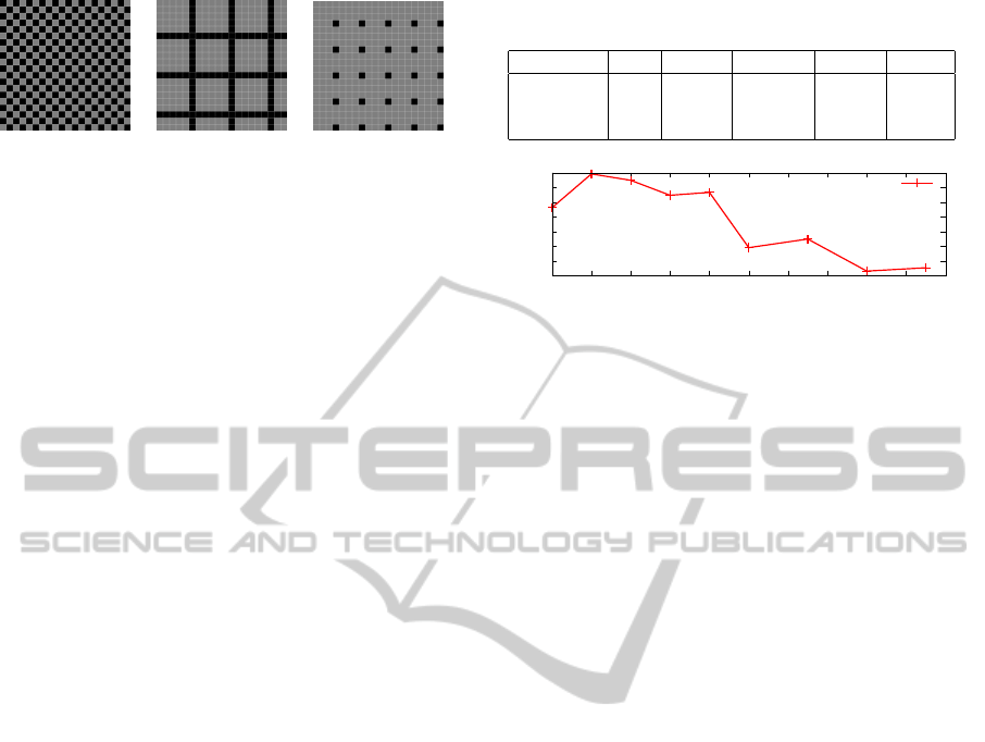
(a) (b) (c)

Figure 5: Cell patterns for histogram sampling. (a) checker-

board pattern using 50 %, (b) 5:1 linear pattern using cca.

36 %, and (c) sparse pattern using 6.25 % of pixels for each

cell.

We recommend uniform sampling of the cell. The

checkerboard pattern is a good option, and the amount

of pixels can be further reduced using other patterns

(Fig. 5).

Cell size should be small enough to having many

of them to build a QR code, so threshold would be

chosen easily for dropping or keeping cell groups. On

the other hand, it has to be large enough to provide re-

liable statistical data for the histogram, at least tens of

pixels for each bin. Papers on visual code localization

suggest empirically (Bodn

ar and Ny

ul, 2012), or us-

ing geometrical approach (Bodn

ar and Ny

ul, 2013),

that optimal tile size is about 1/3 of the smaller di-

mension of the expected visual code in case of fea-

tures based on image partitioning. The number of his-

togram bins can also be tuned to fulﬁll reliability and

robustness. Too many histogram bins leads to sensi-

tivity to noise, while choosing too few bins result in

losing the feature. We recommend about 8 to 16 bins

for 8-bit grayscale images. The range of expected

code size, the desired number of bins and the mean

pixel count falling into each bin determines the usable

pattern and block size for detection. From another

point of view, the number of bins, the expected mean

pixel count and the block coverage ratio of the cho-

sen pattern deﬁnes the size of the smallest detectable

visual code.

3 EVALUATION AND RESULTS

The proposed method has been evaluated on 98 ar-

bitrarily acquired images using a 3.2 Mpx Huawei

smartphone camera, without auto-focus capabilities

and ﬂash. Unit size of the QR codes present in those

images were about 6–10 pixels, overall QR code size

was cca. 200 ×200 pixels. Image size was 800 × 600

pixels. An example from this set is shown on Fig. 1.

Even lighting is preferred, but not necessary for the

captured images. Images with uneven lighting has

to be pre-processed with local contrast stretching per-

formed in each block. Color images are also preferred

Table 2: Evaluation of the FIS on different block offsets and

40 px block size.

Block offset T

opt

F-score Precision Hit rate AUC

10 px 0.62 0.8124 0.8349 0.8766 0.8934

20 px 0.62 0.8124 0.8354 0.8773 0.8938

40 px 0.62 0.8584 0.8377 0.8802 0.8709

0.72

0.74

0.76

0.78

0.8

0.82

0.84

0.86

20 40 60 80 100 120 140 160 180 200 220

F-score

Figure 6: Performance of the FIS with respect to block size.

for the saturation rule, that can be replaced by the rule

based on histograms in case of grayscale input im-

ages. Geometrical distortions of the code leave the

above features intact, as long as there are sufﬁcient

blocks to form a ROI in the feature matrix.

A Core 2 Duo 3.00 GHz CPU could process

roughly 20 of these images each second, so real-

time localization is possible. The FIS can be fur-

ther optimized using ramp terms instead of ZMF

and SMF. HSV channel images can be easily com-

puted from RGB channels using V

= max(R

)

and S

= (max(R

) −min(R

))/V

for all

i ∈ I(x,y). Furthermore, using a lookup table instead

of online calculations is also possible, since the table

only would take one megabyte of data using precision

of two decimals, which is sufﬁcient for the task.

As the ﬁrst test, various block sizes were eval-

uated to determine optimal block size ratio accord-

ing to the expected QR code size, not involving his-

tograms. Results show that optimal block size is rang-

ing from about 20 to 35 percent of the QR code size

(Fig. 6). Performance measures were based on the

Jaccard measure. Choosing too small block size leads

to performance drop, since the attributes computed

from the blocks become less reliable, while too large

block sizes also decrease accuracy, since then only

a smaller number of blocks are fully covered with a

QR code part, and partially covered blocks are also

harder to classify. Instead of a fully universal, multi-

scale solution (Lindeberg, 1993), speciﬁc resolutions

and block sizes lead to more accurate implementa-

tions that can be important on embedded systems.

The effect of the block overlap to performance

was also evaluated and is shown in Table 2. Block

size was set to 40 px and each block was offset by 10,

20 and 40 px (meaning no overlap), respectively. Re-

sults show that evaluation with overlapping blocks did

not increase performance.

Performance of the FIS has also been evaluated

on code types other than QR codes. We assem-

LocalizationofVisualCodesusingFuzzyInferenceSystem

349

Table 3: FIS performance on different visual code types.

1D-S denote for stacked barcodes.

Type Dim. Block size Precision Hit rate F-score

QR 2D 50 px 0.9224 0.9353 0.9288

Aztec 2D 50 px 0.8738 0.9639 0.9167

Data matrix 2D 50 px 0.9214 0.9399 0.9305

Codablock 1D-S 20 px 0.7136 0.7287 0.7210

PDF417 1D-S 20 px 0.7277 0.7007 0.7140

bled four test sets containing Aztec codes and Data

matrix codes as two-dimensional, and Codablock

and PDF417 codes as stacked one-dimensional types.

Stacked 1D codes, like real 2D ones, embed informa-

tion along both axes. These synthetic examples are

built with computer-generated codes containing ran-

dom letters and numerals of the alphabet. The code

was placed on a negative image, with random rota-

tion. Gaussian smoothing and noise have been grad-

ually added to the images. The σ for the Gaussian

kernel was varied in the range [0,3]. A noise im-

age (I

) was generated with intensities ranging from

[-127, 127] following normal distribution, and added

gradually to the original 8-bit image (I

) as I = αI

(1 − α)I

, with α ranging [0, 0.5]. The noise was

added to the image using saturation arithmetic.

Results show that real 2D codes behave simi-

larly to QR codes, despite their structural differ-

ences (Table 3). One-dimensional stacked codes had

smaller height, therefore the block size has been set to

smaller, however, localization performance was infe-

rior to that for real 2D codes. This is probably due to

the fact that in real 2D codes row and column patterns

are similar while in stacked 1D codes they are quite

different. The input variables used for the FIS are ba-

sically direction-invariant and thus suit better for 2D

codes.

To compare efﬁciency of the proposed method to

other implementations from the state of the art, we

evaluated it on two public databases, from S

os et

al. (S

os and Fl

orkemeier, 2013), and Dubsk

a et al.

(Dubsk

a et al., 2013), respectively.

os et al. made their set using 200 blurry images

acquired by iPhone5, without auto-focus. The evalu-

ation of the FIS on this set was performed with mi-

nor modiﬁcations of the original input terms based on

sample images of the set. The graydist avg attribute

had its perfect SMF term adjusted to SMF(0.25,0.5),

since images of this set had poor contrast due to the

heavy blur present. Mean intensity of the blocks

were also higher, so the Gaussian term representing

the perfect membership function has been modiﬁed

to G(m = 0.61, σ = 0.09). SMF term regarding satu-

ration could be set to SMF(0.075, 0.19), which led to

a stricter saturation rule than the one of our original

test set. Results in Table 4 show performance of the

Table 4: Results of the proposed method on the S

os et al.

and Dubsk

a et al. data sets.

Data set Precision Hit rate F-score

os et al. (Original FIS) 0.5938 0.5224 0.5558

os et al. (Median ﬁltered) 0.5890 0.6018 0.5953

Dubsk

a et al. Set-1 0.6165 0.5036 0.5544

Dubsk

a et al. Set-2 0.9288 0.9513 0.9399

(a)

(b) (c)

Figure 7: Output stabilization of a sample image from the

os et al. set. (a) original image, (b) feature image, (c)

median ﬁltered feature matrix.

FIS on this test set for the original algorithm, and one

with median ﬁlter as post-processing. Fig. 7 shows an

example of this data set with the corresponding fea-

ture images.

The second public database by Dubsk

a et al. con-

tained two similar sets of QR code images, sur-

rounded with text in a scene having low saturation

in general. The ﬁrst set has 410 high-resolution

(2560 × 1440 px) images with uneven lighting con-

ditions, high grades of distortion and minor blur

(Fig. 8(a)). The second test set has 400 low-resolution

(604 × 402 px) images with smaller grades of distor-

tion and more even illumination, but having less light

in general, thus producing darker images (Fig. 8(c)).

For the ﬁrst set of this database, FIS had to be set

for larger tolerances for the perfect term of blockavg,

and graydist avg was also set to lower acceptance

value, deﬁned by SMF(0.25,0.3). However, images

of the ﬁrst set have shown so high variability for the

mean intensities within blocks, contrast and QR code

size that the designed FIS could not be generalized

enough to classify all samples well. We can overcome

this issue using adaptive thresholding or local contrast

stretching, at the cost of more computation time. On

the second data set, with a chosen block size 50 px,

FIS terms of positive response could be tuned more

easily, therefore the proposed method performed bet-

ter with respect to both precition and hit rate (Table 4).

VISAPP2015-InternationalConferenceonComputerVisionTheoryandApplications

350

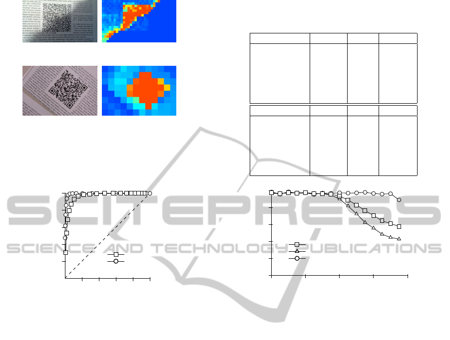
(a) (b)

Figure 8: Examples of the Dubsk

a et al. Set-1 (a) and Set-

2 (c), and their feature images (b) and (d), respectively. In

both cases the block size was 60 px, but the size of the ﬁrst

image is much higher than that of the second.

0.2 0.4 0.6 0.8 1

0.2

0.4

0.6

0.8

1 - Speciﬁcity

Sensitivity

Synthetic data

Real data

Figure 9: Efﬁciency of the proposed algorithm according to

different thresholds, visualized in ROC space.

3.1 Performance Measures of the Cell

Histogram Feature

Four variants of the histogram-based feature was

evaluated separately from the FIS, each named af-

ter the pattern they use for building the cell his-

tograms (HIST-FULL uses all pixels, HIST-CHK,

HIST-LIN and HIST-SPA uses the checkerboard, lin-

ear and sparse patterns, respectively), and compared

to the works of Ohbuchi et al. (Ohbuchi et al., 2004)

and Lin et al. (Lin and Lin, 2013).

The effect of chosen threshold T to efﬁciency, us-

ing HIST-FULL, is shown in Fig. 9. AUC for syn-

thetic and real data are 0.9924 and 0.8938, respec-

tively. Sensitivity drops below 1.0 at T = 0.73, and

F-measure peaks at T = 0.86. For industrial setups,

where localization of all codes is crucial, we recom-

mend T ≈ 0.8, since sensitivity is still 99 % and pre-

cision is about 50 %. The behavior for chosen thresh-

old and noise level is similar in all chosen patterns.

Fig. 10 shows that noise has no signiﬁcant effect to

false positive rate, it only drops sensitivity at higher

rates. Detailed results are shown in Table 5 for syn-

thetic and real images of the database.

Table 5: Performance measures of the proposed algorithm

using different cell patterns, compared to other localization

approaches (Ohbuchi et al., 2004; Lin and Lin, 2013).

Synthetic images Precision Recall Accuracy

REF-OHBUCHI 1.0000 0.837 0.8730

REF-LIN 0.9340 0.9490 0.8890

HIST-FULL 0.8320 0.9382 0.9732

HIST-CHK 0.8576 0.9035 0.9737

HIST-LIN 0.6625 0.9389 0.9426

HIST-SPA 0.6729 0.9014 0.9429

Real images Precision Recall Accuracy

REF-OHBUCHI 0.9500 0.8750 0.8360

REF-LIN 0.9400 0.8930 0.8450

HIST-FULL 0.7672 0.9011 0.9630

HIST-CHK 0.7677 0.9016 0.9631

HIST-LIN 0.7662 0.9056 0.9632

HIST-SPA 0.7652 0.9005 0.9627

0.05 0.1 0.15 0.2 0.25

0.2

0.4

0.6

0.8

Noise level

Precision

Sensitiviy

F-measure

Figure 10: Precision, Sensitivity and F-measure according

to noise level, using 0.86 as threshold.

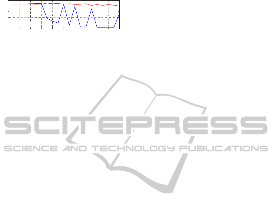
3.2 Using Partial Block Information

As in the case of histograms, the number of read pix-

els can be limited to speed up FIS processing. Fig. 11

shows results of the sparse data evaluation. The x

axis represents the sampling factor, which means that

only every n-th pixel is read from both the rows and

columns, so the amount of pixels used to calculate

the FIS input variables, is reduced by a factor of

. This partial block information does not introduce

more false positives, it only affects the hit rate by ren-

dering the only rule of positive response unreliable

in the FIS. Results also show that the chosen sam-

pling interferes with the unit size of the QR code. Hit

rate temporally rises while reading only every 10th,

12th and 15th pixel, since it gives a more reliable

block sampling for attribute computation, which is

caused by the cca. 6 px unit size of the used QR

codes in those images. Choosing the sampling factor

k · unitsize/2,(k ∈ Z) is more likely to sample most

QR code units from the same position, like close to

center of unit, or close to their perimeter. However,

we cannot make any assumptions on expected QR

unit size on arbitrarily acquired images, therefore us-

LocalizationofVisualCodesusingFuzzyInferenceSystem

351

0.2

0.4

0.6

0.8

0 2 4 6 8 10 12 14 16 18 20

precision

hit rate

Figure 11: Performance of the FIS on sparse data. Values

of the x axis mean that only every n-th pixel is read with

respect to rows and columns.

ing large sampling factor is considered unreliable in

general. Furthermore, chosen block size gives an up-

per limit to sampling, since calculation of the FIS in-

put attributes are based on statistics and therefore re-

quire tens of pixels for each block. In order to stabi-

lize the FIS output by region compactness, we could

take adjacent blocks into consideration. To avoid

large increase of computation time, evaluation of this

condition is recommended to be performed outside

the FIS, in the feature matrix. Small “holes” of the

matrix, values surrounded by blocks of high values,

are likely to be false negatives. Similarly, “lonely”

blocks of high value can be safely zeroed out, since

they probably do not participate in any QR code can-

didate. Morphological ﬁltering, or as a simpler opera-

tion, median ﬁltering are suitable for this task (Fig. 7).

In most cases, the latter seems sufﬁcient according to

experimental results, however, using morphology at

this step is also acceptable, since the size of the fea-

ture matrix is only a small fraction of that of the orig-

inal input image.

4 CONCLUDING REMARKS

In this paper, we have shown that Fuzzy Inference

Systems can be used to rapidly localize QR codes in

the image domain. We have examined efﬁciency of

Fuzzy Inference Systems that has membership func-

tions created by preliminary assumptions based on

statistics of a few sample images of the expected sce-

nario. For industrial setups, making this assumption

is easy, since variability of the content is smaller. For

smartphone applications, parameters can be tuned us-

ing camera properties. Performance has been evalu-

ated on public test image sets.

Block size and amount of overlap has also been

evaluated, thus giving information about the robust-

ness of the approach. FIS can be replaced by lookup

tables that leads to constant-time evaluation. Calcu-

lation of the input features can be further accelerated

using approximations with only a subset of intensity

values. These properties can make FIS-based local-

ization a preferred choice over other algorithms.

The proposed algorithm can also be used to efﬁ-

ciently localize other popular two-dimensional code

types as well, like Aztec codes or Data matrix codes,

without major modiﬁcation.

ACKNOWLEDGEMENT

This publication is supported by the European Union

and co-funded by the European Social Fund. Project

title: Telemedicine-oriented research activities in

the ﬁelds of mathematics, informatics and medi-

cal sciences. Project number: T

AMOP-4.2.2.A-

11/1/KONV-2012-0073.

REFERENCES

Belussi, L. F. F. and Hirata, N. S. T. (2011). Fast QR code

detection in arbitrarily acquired images. In Graphics,

Patterns and Images (Sibgrapi), 2011 24th SIBGRAPI

Conference on, pages 281–288.

Bodn

ar, P. and Ny

ul, L. G. (2012). Improving barcode de-

tection with combination of simple detectors. In The

8th International Conference on Signal Image Tech-

nology (SITIS 2012), pages 300–306.

Bodn

ar, P. and Ny

ul, L. G. (2013). A novel method for

barcode localization in image domain. In Image Anal-

ysis and Recognition, volume 7950 of Lecture Notes

in Computer Science, pages 189–196.

Chu, C.-H., Yang, D.-N., Pan, Y.-L., and Chen, M.-S.

(2011). Stabilization and extraction of 2D barcodes

for camera phones. Multimedia Systems, 17:113–133.

Dubsk

a, M., Herout, A., and Havel, J. (2013). Real-time

precise detection of regular grids and matrix codes.

Journal of Real-Time Image Processing, pages 1–8.

Lin, D.-T. and Lin, C.-L. (2013). Automatic location

for multi-symbology and multiple 1D and 2D bar-

codes. Journal of Marine Science and Technology,

21(6):663–668.

Lindeberg, T. (1993). Scale-space theory in computer vi-

sion. Springer.

Ohbuchi, E., Hanaizumi, H., and Hock, L. A. (2004).

Barcode readers using the camera device in mobile

phones. In Cyberworlds, 2004 International Confer-

ence on, pages 260–265.

Rubner, Y., Tomasi, C., and Guibas, L. J. (2000). The earth

mover’s distance as a metric for image retrieval. Inter-

national Journal of Computer Vision, 40(2):99–121.

os, G. and Fl

orkemeier, C. (2013). Blur-resistant joint

1D and 2D barcode localization for smartphones. In

Proceedings of the 12th International Conference on

Mobile and Ubiquitous Multimedia, MUM ’13, pages

11:1–11:8, New York, NY, USA. ACM.

Swain, M. J. and Ballard, D. H. (1991). Color indexing. Int.

J. Comput. Vision, 7(1):11–32.

VISAPP2015-InternationalConferenceonComputerVisionTheoryandApplications

352