GPU Ray-traced Collision Detection

Fine Pipeline Reorganization

Franc¸ois Lehericey, Val

erie Gouranton and Bruno Arnaldi

INSA de Rennes, IRISA, Inria, Campus de Beaulieu, 35042 Rennes cedex, France

Keywords:

Collision Detection, Narrow-phase, GPU Computing.

Abstract:

Ray-tracing algorithms can be used to render a virtual scene and to detect collisions between objects. Numer-

ous ray-tracing algorithms have been proposed which use data structures optimized for speciﬁc cases (rigid

objects, deformable objects, etc.). Some solutions try to optimize performance by combining several algo-

rithms to use the most efﬁcient algorithm for each ray. This paper presents a ray-traced collision detection

pipeline that improves the performance on a graphicd processing unit (GPU) when several ray-tracing algo-

rithms are used. When combining several ray-tracing algorithms on a GPU, a well-known drawback is thread

divergence among work-groups that can cause loss of performance by causing idle threads. In this paper we

avoid branch divergence by dividing the ray tracing into three steps with append buffers in between. We also

show that prediction can be used to avoid unnecessary synchronizations between the CPU and GPU. Applied

to a narrow-phase collision detection algorithm, results show an improvement of performance up to 2.7 times.

1 INTRODUCTION

Collision detection (CD) is an important task in vir-

tual reality (VR). From a set of objects, we need to

know those which collide. Nowadays collision is one

of the main bottlenecks in VR applications due to the

complexity of environments we want to simulate and

the real-time constraint required by VR. We need to

simulate large environments that can count millions

of objects. And we want to include complex objects

that can be deformable, undergo topology changes or

be ﬂuids.

To handle such a work load, collision is generally

divided into two phases: broad-phase and narrow-

phase. The broad-phase takes the whole set of objects

from the environment and provides a set of pairs of

objects that might collide. The narrow-phase takes

these pairs and outputs the ones that actually col-

lide. This paper focuses on the narrow-phase which

is nowadays the most time-consuming phase.

Recent approaches use GPGPU (general-purpose

computing on graphics processing units) to take ad-

vantage of the high computational power of recent

GPUs. Parallel implementation of the broad-phase

sweep and prune algorithm on GPUs improve per-

formance by orders of magnitude (Liu et al., 2010).

The narrow-phase can also be implemented on a GPU

(Pabst et al., 2010).

In the literature four categories of narrow-phase

algorithms are studied, including image-based algo-

rithms that uses rendering techniques to detect colli-

sions. As GPUs are designed especially for render-

ing, image-based methods are well suited for GPGPU

implementations. In particular ray-tracing algorithms

can be used and several ones can be combined

to improve performance (Lehericey et al., 2013a).

When implementing several ray-tracing algorithms

on GPUs, high branch divergence in the execution

can lead to underuse of the GPU and reduced perfor-

mance.

Main Contributions: we present a new pipeline or-

ganization of the narrow-phase for ray-traced colli-

sion detection. The goal of our pipeline is to minimize

thread divergence on GPUs to improve performance.

Our pipeline is designed to be able to integrate sev-

eral ray-tracing algorithms without causing overhead.

We then present a prediction method to avoid CPU-

GPU synchronization between steps of the pipeline to

further improve performance.

This paper is arranged as follows. The follow-

ing section provides a reviex of the relevant literature.

Section 3 presents our ray-traced collision pipeline.

Section 4 shows how prediction can be used to avoid

unnecessary synchronization between the CPU and

GPU. Implementation and results are discussed in

Section 5. Section 6 concludes this paper.

317

Lehericey F., Gouranton V. and Arnaldi B..

GPU Ray-traced Collision Detection - Fine Pipeline Reorganization.

DOI: 10.5220/0005299603170324

In Proceedings of the 10th International Conference on Computer Graphics Theory and Applications (GRAPP-2015), pages 317-324

ISBN: 978-989-758-087-1

 2015 SCITEPRESS (Science and Technology Publications, Lda.)

2 RELATED WORK

This section focuses on the literature on CD which is

most pertinent to our work, in particular image-based

algorithms for the narrow-phase. For an exhaustive

overview on CD, readers should refer to surveys such

as (Teschner et al., 2005; Kockara et al., 2007).

2.1 Image-based Collision Detection

Image-based algorithms use rendering techniques to

detect collisions. These methods are often adapted for

GPUs, which are processors designed for rendering.

Image-based methods can be used to perform colli-

sion detection on rigid and deformable bodies. These

techniques usually do not require any pre-processing

steps which makes them suitable for dynamically de-

forming objects. Image-based algorithms can either

use rasterization or ray-tracing techniques.

Rasterization can be used to compute a layered

depth image (LDI) which can be post-processed to

detect collisions (Allard et al., 2010). The CInDeR

algorithm (Knott, 2003) uses rasterization to implic-

itly cast rays from the edges of an object and counts

how many object faces the ray passes through. If the

result is odd then there is collision; otherwise there is

no collision. (Heidelberger et al., 2003; Heidelberger

et al., 2004) take three-dimensional closed objects and

output the intersection volume without the needs of

any data structures making it suitable for deformable

objects. The main drawback of these techniques is the

discretization of the space through rendering that in-

duces approximations and may lead to the omission

of small objects.

Ray-tracing algorithms can be used to overcome

these approximations. (Wang et al., 2012) show that

ray tracing can be used to compute a LDI with a

higher resolution around small objects by increasing

the density or rays locally to increase the precision.

(Hermann et al., 2008) detect collisions by casting

rays from each vertex of the objects. Rays are cast

in the inward direction; the ones that hit another ob-

ject before leaving the source object detect a collision.

Before casting a ray, the ones that are outside the in-

tersection of the bonding volumes are dropped since

they cannot collide.

Based on Hermann et al.’s algorithm, (Lehericey

et al., 2013a; Lehericey et al., 2013b) introduced

an iterative ray-traced collision detection algorithm

(IRTCD). This method combines two different ray-

tracing algorithms; a full and an iterative algorithm

that are respectively used for high and small displace-

ments between objects. The full algorithm can be

any existing ray-tracing algorithm. The iterative al-

gorithm is a fast ray-tracing algorithm that exploits

spatial and temporal coherency by updating the previ-

ous time-step. These algorithms can be used on GPUs

for improved performance.

2.2 GPU Computing

Several methods consider the GPU as a streaming

processor. As GPUs are massively parallel proces-

sors, computations should be arranged to be made

parallel (Nickolls and Dally, 2010).

When code runs on a GPU, the same function

(called kernel) is called by multiple threads (called

work-item) on different data. Work-items do not run

independently but in a group (called work-group); in

a work-group, work-items run in a single instruction,

multiple data way. On a conditional branch, if the

work-items diverge among a work-group, each branch

runs serially. This phenomena is called thread diver-

gence and reduces performance (Zhang et al., 2010).

One case of thread divergence is having a sparse

input, in which case some work-items have nothing to

do and are idle in a work-group while the other work-

items ﬁnish. Collision-streams (Tang et al., 2011)

use stream compaction to avoid kernel execution on

sparse inputs. Collision detection is divided into sev-

eral steps and streaming compaction is used between

steps to ensure dense input for each kernel.

2.3 Synthesis

Ray-traced collision detection can be used on GPUs

to achieve high performance on complex scenes. In

a simple scenario only one ray-tracing algorithm can

be used to resolve collisions. But in complex scenes

with objects of different nature we can employ sev-

eral ray-tracing algorithms to optimize each nature of

object. With rigid objects we can use algorithms with

complex data structures. With deformable objects we

need data structures that can be updated at each time-

step. In the case of topology changes we need to re-

construct the ray-tracing data structures occasionally.

Iterative ray-tracing can be used to accelerate all of

these algorithms.

In complex scenes where all these properties

are represented, combining several ray-tracing algo-

rithms improves performance. In such situations, the

need of a narrow-phase that can easily manage di-

verse ray-tracing algorithms without losing perfor-

mance emerges.

GRAPP2015-InternationalConferenceonComputerGraphicsTheoryandApplications

318

3 RAY-TRACED CD PIPELINE

To perform our ray-traced CD method there are sev-

eral ray-tracing algorithms available in the literature.

We selected three algorithms. We qualify the two ﬁrst

ones as ‘full’ ray-tracing algorithms; these algorithms

can be used at any time. The third algorithm, called

iterative, requires speciﬁc conditions.

The ﬁrst full algorithm is a stackless bounding

volume hierarchy (BVH) traversal. This algorithm

uses an accelerative structure and can be used for

rigid objects. The second full algorithm is basic ray-

tracing. This algorithm does not use any additional

accelerative structures and can be used for deformable

objects. If we used the stack-less BVH traversal algo-

rithm or deformable objects, we would need to update

the accelerative structure at each time-step.

The third ray-tracing algorithm which we do not

qualify as ‘full’ is the iterative ray-tracing algorithm.

This algorithm is incremental and updates the previ-

ous time-step. This algorithm cannot be used at any

time because it needs an extra input to work; this extra

input is the reference of the last hit triangle in the pre-

vious time-step (called temporal data in the remainder

of this document). The iterative algorithm needs a full

ray-tracing algorithm to ﬁrst create temporal data and

then it can be used to replace the full algorithm in the

following steps. We can use the iterative algorithm

as long as relative displacement between the ray and

target of the ray remain small. When temporal data is

available, the iterative algorithm is faster than the two

previous ones and should be preferred.

Before executing the ray-tracing we can perform

simple culling tests to reduce the total number of rays

to cast. If the origin of the ray is outside the bounding

volume of the target, we can remove that ray because

it cannot be inside the target. For rays using the iter-

ative algorithm, we test if temporal data is available

from the last step. If no temporal data is available we

can drop the vertex because the iterative algorithm re-

quires temporal data. The absence of temporal data

indicates that at the previous time-step no collision

was detected for this vertex and no prediction indi-

cated a possible future collision.

When combining several ray-tracing algorithms

on GPUs, the naive implementation consists of exe-

cuting one large kernel that implements all the ray-

tracing algorithms with a switch to select which algo-

rithm to use for each vertex. This naive implemen-

tation will cause thread divergence for two reasons.

First, all the ray-tracing algorithms are executed by

the same kernel; this adds a branch divergence on the

execution of each ray trace. Each work-group that ex-

ecutes more than one algorithm will execute them se-

quentially. Second, in a context where we can safely

cull some vertices to reduce the amount of compu-

tation, this naive implementation will initiate work-

items that ﬁnish immediately. These work-items will

then be idle while the other work-items of the work-

group ﬁnish.

This section presents our pipeline distribution of

tasks to improve the performance of ray-traced col-

lision detection on GPUs. Subsection 3.1 gives an

overview of the pipeline and the three steps. Subsec-

tion 3.2, 3.3 and 3.4 detail the three steps: per-pair,

per-vertex and per-ray steps.

3.1 Pipeline Organization

To achieve collision detection our narrow-phase

pipeline must perform several tasks: Apply a mea-

surement of displacement on the pair of objects to

decide if we use a full or the iterative ray-tracing algo-

rithm. Cull vertices with simple criteria to avoid un-

necessary ray-tracing. Execute the ray-tracing from

the remaining vertices; the algorithm depends on the

nature of the object or if we decided to use the itera-

tive algorithm.

The displacement measurement can be applied

globally on a pair of rigid objects and needs to be ap-

plied per vertex when a deformable object is present

to take into account internal deformations. Pairs (or

vertices) classiﬁed with small displacement will use

the iterative ray-tracing algorithm.

Vertex culling uses a drop criterion to remove ver-

tices that do not need to be tested with ray-tracing be-

cause a simple test can discard collision. For the ver-

tices classiﬁed as evidencing displacement, we check

if the vertex is inside the intersection of the bounding

volumes of the two objects of the pair. For the ver-

tices classiﬁed as showing small displacement we test

the presence of temporal data.

Ray-tracing is executed for each of the remain-

ing vertices. We use the iterative algorithm when se-

lected; otherwise, we use an algorithm that depends

on the nature of the target of the ray-tracing.

These tasks show that the narrow-phase must pro-

cess data at three different levels of granularity: per-

pair, per-vertex and per-ray granularity. The goal of

this decomposition is to avoid branch divergence and

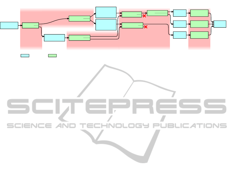
ensures a dense input at each step. Figure 1 gives an

overview of the pipeline organization.

Append buffers are used between each step to

store data. The kernel preceding the append buffer

ﬁlls it. Each entry of the buffer generates threads in

the following kernel. The main purpose is to guar-

antee a dense input to the following kernel and avoid

idle threads.

GPURay-tracedCollisionDetection-FinePipelineReorganization

319

Broad Phase

Pair List

contains

only rigid?

yes

Small

Displacement

Pair List

Delayed Test

Pair List

High

Displacement

Pair List

inside BV

intersection?

yes

temporal

data available?

yes

BVH

Ray List

Iterative

Ray List

Basic

Ray List

target

is ?

rigid

deformable

BVH

ray-tracing

Iterative

ray-tracing

Basic

ray-tracing

Contact

Points

One thread

per pair

One thread

per vertex

One thread

per ray

high

small

relative

displacement

Buﬀer Kernel

high

small

relative

displacement

nature

selection

displacement

measurement

drop

criterion

nature

selection

ray-tracing

Figure 1: Pipeline organization of the narrow-phase. The narrow-phase starts from the list of pairs of objects detected by

the broad-phase. The ﬁrst step is applied on the pair and we separate them into three categories: rigid pairs with small

displacement, rigid pairs with high displacement and deformable pairs. The second step is applied on the vertices of the

objects of the pairs; we select which ray-tracing algorithm to use depending on the nature of the objects and the result of the

displacement measurement. The last step is applied on the rays and is the execution of the ray-tracing algorithms.

In the following subsections (3.2, 3.3 and 3.4) we

detail the content of the three steps.

3.2 Per-pair Step

The per-pair step starts from the list of pairs of objects

provided by the broad phase. In this step one thread

corresponds to one pair.

First we split the pairs into two categories: those

which contain only rigid objects and those which con-

tain deformable objects. This separation is applied

because the criterion to decide if we use a full or the

iterative algorithm is different.

For the pairs with only rigid objects we apply at

this stage a displacement criterion to separate those

with high displacement that will use a full ray-tracing

algorithm and the ones with small displacement that

will use the iterative algorithm. We cannot apply

a displacement criterion on the pairs that contain at

least one deformable object in this stage. In such

cases displacement needs to be measured locally to

take into account internal deformations.

3.3 Per-vertex Step

The per-vertex step starts from each list of pairs con-

structed in the per-vertex step. In this step one thread

is executed for each vertex of each object of each pair.

For the pair containing deformable objects, we can

now apply a displacement measurement on the ver-

tices to separate the ones with small displacement that

will use the iterative algorithm and the others that will

use a full algorithm.

Then we apply a drop criterion on the vertices to

cull the ones that can be safely discarded. The crite-

rion is different for vertices using a full algorithm and

vertices using the iterative algorithm. For the vertices

that use a full algorithm, we check if the vertex is in-

side the intersection of the bounding volumes of the

two object of the pair. If not, we can drop this ver-

tex as it cannot collide. For the vertices that use the

iterative algorithm, we test if temporal data is avail-

able from the preceding step. If no temporal data is

available we can drop the vertex.

After applying the drop criterion, each remaining

vertex generates a ray that will be cast on the other

object of the pair; the parameters needed to cast these

rays are stored in three buffers. Vertices using the it-

erative algorithm ﬁll the list of rays for the iterative

ray-tracing algorithm. Rays generated from vertices

using a full algorithm need to be separated into two

categories: rays cast to a rigid object use a stackless

BVH ray-tracing algorithm; rays cast to a deformable

object use the basic ray-tracing algorithm.

3.4 Per-ray Step

The per-ray step starts from each list of rays and exe-

cutes the ray-tracing. Each thread casts one ray.

The BVH ray list uses the stackless BVH traversal

algorithm. This algorithm uses a BVH as an accel-

erative ray-tracing structure (Wald et al., 2007) with

a stackless traversal adapted for GPUs (Popov et al.,

2007). The basic ray list uses the basic ray-tracing

algorithm. This algorithm does not use any acceler-

ative structure; for each ray we iterate through each

triangle. This method has high complexity but does

not necessitate any accelerative structures that would

need to be updated after each deformation. The iter-

ative ray list uses the iterative ray-tracing algorithm

(Lehericey et al., 2013a). This algorithm can be used

on both rigid and deformable objects.

Each ray-tracing algorithm is implemented and

executed in a separate kernel to avoid branch diver-

gence in the GPU. The ray-tracing algorithms output

contact points for the physics response.

GRAPP2015-InternationalConferenceonComputerGraphicsTheoryandApplications

320

task A task B

task B

task A task B

task B

enqueue

task A

enqueue

task B

enqueue

task B

read

completion

CPU

GPU

CPU

GPU

synchronization

time

extra work-items

begin

end

exact workload

workload prediction

enqueue

task A

enqueue

task B

enqueue

task B

read completion

asynchronously

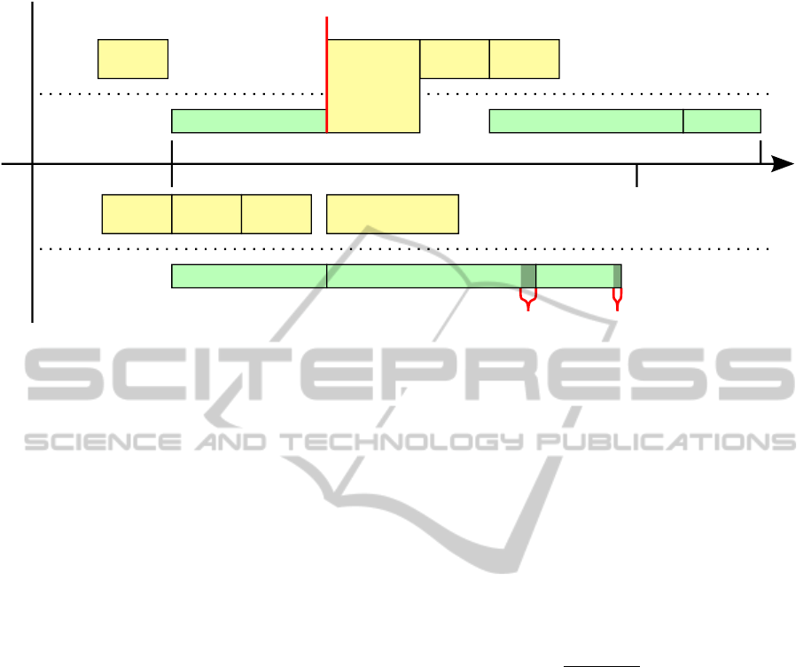
Figure 2: Comparison of the timeline of events between “exact workload” and “workload prediction”. In this example a task,

A, ﬁlls an append buffer and two tasks, B

and B

, use it. On the top part we execute the B

and B

tasks with the optimal

work size but the GPU spends time in idle mode due to a synchronization. On the bottom part we use a prediction of the

completion to schedule the tasks at the cost of some empty work-items.

4 BUFFER COMPLETION

PREDICTION

Along the narrow-phase we need to know the number

of elements contained in each append buffer (which

we will refer to as completion in the rest of this sec-

tion). For each append buffer we need to know a priori

the completion to allocate sufﬁcient space and a pos-

teriori to know how many threads must be launched

in the following kernels. But these completion values

are unavailable a priori and stored in the GPU mem-

ory a posteriori. To avoid extra computations or syn-

chronizations that would lower the performance, we

can rely on predictions.

In this section we will ﬁrst explain, in subsec-

tion 4.1, our general prediction scheme and then we

will apply this prediction scheme to the append buffer

sizes and on the workload in subsection 4.2 and 4.3.

4.1 Generic Prediction

Let N

be the number of elements contained in an ap-

pend buffer at the current time-step, and N

t−1

at the

previous time-step. p(N

) is the predicted value at the

time-step t.

We have access to N

t−1

, i.e. the exact count that

should have been used in the previous time-step. This

value can be retrieved asynchronously with no ex-

tra cost. To predict the evolution of the value, we

rely on the evolution of the number of pairs issued

by the broad-phase which gives an indication on the

evolution of the global workload. Let nbPairs

(and

nbPairs

t−1

) be the number of pairs detected by the

broad-phase at the time-step t (and t − 1).

Equation 1 gives a prediction value p(N

). We

take as input the real value at the previous time-step,

t−1

. We weight the value with the evolution of the

number of pairs that give us an indication of the evo-

lution of the workload. And we multiply the result

with a conﬁdence level of at least 1 to take into ac-

count variability.

p(N

) = N

t−1

nbPairs

t−1

× con f idence (1)

At the end of the time-step we can asynchronously

retrieve the real value N

and compare it with the

prediction p(N

) to check if the prediction was high

enough. If the prediction was too low we have two

strategies. The simplest one is to ignore the error and

continue the simulation. This solution will cause er-

rors in the simulation but will be suitable for real-time

applications. The second solution is to backtrack the

simulation and use the real values. This will achieve

a correct simulation and will be preferred for ofﬂine

simulations.

4.2 Buffer Size Prediction

Before we launch a kernel that will ﬁll an append

buffer we need to know a priori the number of ele-

ments that will be inserted to allocate sufﬁcient space.

To get this number we could execute the kernel twice:

once to get the number of outputs and once to ﬁll the

append buffer.

GPURay-tracedCollisionDetection-FinePipelineReorganization

321

We can use prediction to avoid the ﬁrst execution.

We apply the prediction equation to evaluate the size

of the append buffer. We can use a large value of con-

ﬁdence in these predictions as it does not affect com-

putation size but does affect buffer size.

4.3 Workload Prediction

To be able to schedule a kernel that takes as input

an append buffer we need to know the completion of

the buffer to know how many threads to launch. This

completion value is in the GPU memory and the ker-

nel execution is scheduled by the CPU. We have two

solutions to manage this data dependency:

The ﬁrst solution, called exact workload, consists

of reading back the completion from the GPU to the

CPU. Then we can schedule the next kernels with the

exact number of threads. The upper part of Figure

2 shows the timeline of the events on the CPU and

GPU. The major drawback of this method is the syn-

chronization between the CPU and GPU; the GPU is

idle while waiting for the next kernel’s execution.

The second solution, called workload prediction,

does not to rely on the exact completion, but predicts

it. To predict the completion we can apply the pre-

diction equation with a large value of conﬁdence to

minimize the risk of missing some rays. If we run too

many threads, they will immediately exit after check-

ing if their index exceed the completion value stored

in the GPU. The drawback of this method is that large

prediction will lead to empty threads in the GPU, but

these empty work-items will be all grouped in the last

work-groups and thus will not provoke branch diver-

gence. The advantage of this solution is that it does

not trigger any synchronization between the CPU and

GPU as shown in the bottom part of Figure 2.

5 PERFORMANCE EVALUATION

This section presents our experimental environment

and our performance results. First, in 5.1 we present

our experimental setup. Then in subsection 5.2 we

show the performance improvement when using our

ray-traced pipeline method. In subsection 5.3 we

show the performance gain obtained by using predic-

tion. Finally in 5.4 we measure the quantity of errors

introduced by the predictions.

5.1 Experimental Setup

To measure the performance improvements of our

ray-traced narrow-phase we measured the GPU com-

putation time of 10 second simulations executed at 60

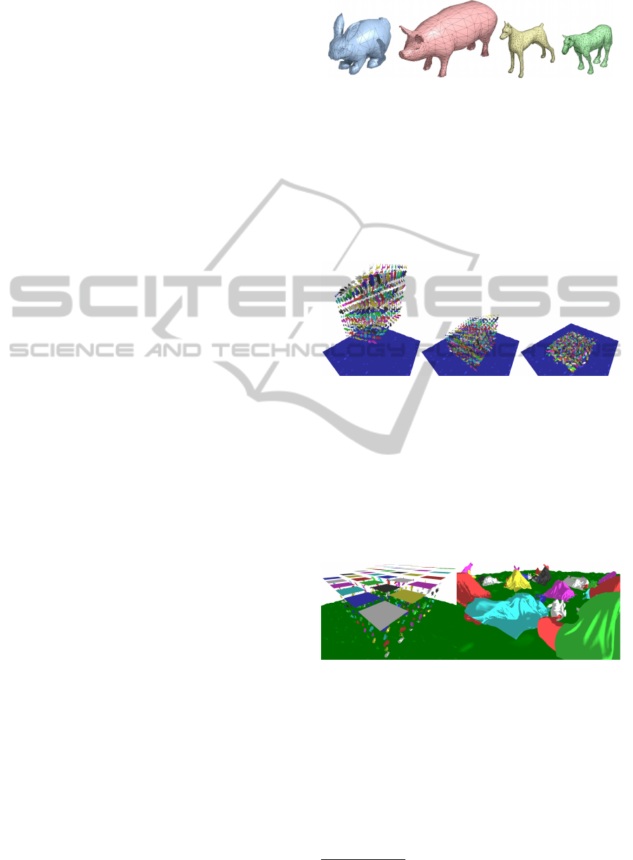
Figure 3: The four rigid objects used in the simulation re-

spectively composed of 902, 2,130, 3,264 and 3,458 trian-

gles.

Hz on two different experimental scenes: ‘rigid ob-

jects’ and ‘rigid and deformable objects’.

In the scene ‘rigid objects’ (see Figure 4) 1,000

rigid non-convex objects fall on an irregular ground.

Four different objects presented in Figure 3 are used

in equal quantities. Up to 10,000 pairs of objects are

tested in the narrow-phase.

Figure 4: ‘Rigid object’ scene: 1,000 concave objects fall

on an irregular ground.

In the scene ‘rigid and deformable objects’ (see

Figure 5) 216 rigid non-convex objects fall on an ir-

regular ground and 36 deformable sheets fall on the

top of them. The rigid objects are the same as in the

ﬁrst scene. The deformable sheets are square shaped

and composed of 8,192 triangles. Up to 860 pairs of

rigid objects and 600 pairs of rigid/deformable objects

are tested in the narrow-phase.

Figure 5: ‘Rigid and deformable object’ scene: 216 concave

objects fall on an irregular ground and 36 deformable sheets

fall over them.

Our experimental scenes were developed with bul-

let physics 3.x

using a GPU. Our narrow phase were

implemented for GPU with OpenCL. All scenes were

executed using an AMD HD 7990.

5.2 Pipeline Performance

To measure the speedup obtained with our narrow-

http://bulletphysics.org/

GRAPP2015-InternationalConferenceonComputerGraphicsTheoryandApplications

322

200

400

600

800

1000

0 1 2 3 4 5 6 7 8 9 10

Narrow-phase computation time (ms)

Time in simulation (s)

without pipeline / without iterative

with pipeline / without iterative

without pipeline / with iterative

with pipeline / with iterative

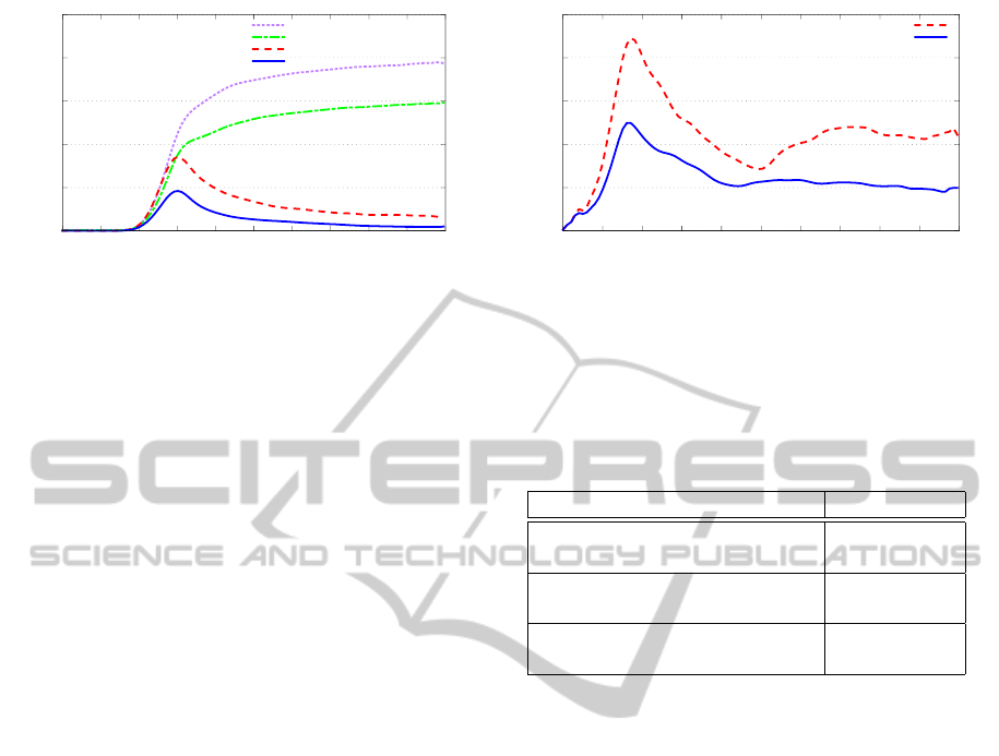
Figure 6: Performance comparison of GPU collision de-

tection with and without our pipeline reorganization in the

scene ‘rigid objects’. With only a full ray-tracing algo-

rithm our method gives an average speedup of 1.31 times

and with the combination of a full and iterative ray-tracing

algorithms our methods gives an average speedup of 2.73

times.

phase pipeline, we compared the GPU computation

time of the narrow-phase while using our pipeline re-

organization and without it.

In the scene ‘rigid objects’ we measured the per-

formance of our pipeline reorganization when using

only the full ray-tracing algorithm (BVH ray traver-

sal) and when using both full and iterative ray-tracing

algorithms. Result are shown in Figure 6.

The ﬁrst result is the speedup obtained when using

our pipeline method with only the full ray-tracing al-

gorithm. We get an average speedup of 1.31 times

when using our pipeline ray-tracing method. This

speedup can be explained by the per-vertex step that

guarantees that the ray-tracing step is executed on

dense data even if the input of the per-vertex step is

sparse.

The second result is the speedup when using our

pipeline method with the combination of full and it-

erative ray-tracing algorithms. The average speedup

when using our pipeline ray-tracing method is 2.73

times. The extra speedup compared to the previous

case come from the execution of each ray-tracing al-

gorithm in a different kernel in the per-ray step which

reduces branch divergence in the GPU.

In the scene ‘rigid and deformable objects’ we

measured the performance of our pipeline reorganiza-

tion when three ray-tracing algorithms are used. Re-

sult are shown in Figure 7. In this scene we get an av-

erage speedup of 1.84 times when using our pipeline

ray-tracing method.

5.3 Workload Prediction

To show the performance improvement when using

our workload prediction strategy, we compared the

GPU computation time of simulation using the work-

load prediction and the exact workload strategies.

0 1 2 3 4 5 6 7 8 9 10

Narrow-phase computation time (ms)

Time in simulation (s)

without pipeline

with pipeline

Figure 7: Performance comparison of GPU collision de-

tection with and without our pipeline reorganization in the

scene ‘rigid and deformable objects’. Our method gives an

average speedup of 1.84 times.

Table 1: Average GPU performance gain between the exact

and prediction strategies for the workload. The workload

prediction strategy is up to 2.84 ms faster per time-step than

the exact workload strategy.

Scenario Average gain

‘Rigid objects’

2.84 ms

Only full ray-tracing

‘Rigid objects’

1.97 ms

Full and iterative ray-tracing

‘Rigid and deformable objects’

2.05 ms

Full and iterative ray-tracing

Table 1 gives the average gain when using the

workload prediction against the exact workload strat-

egy. We measured the gain on both ‘rigid object’

and ‘rigid and deformable objects’ scenes. For the

‘rigid object’ scene we measured the gain when us-

ing only the full ray-tracing algorithm and when using

both full and iterative ray-tracing algorithms. The re-

sults show that the workload prediction strategy is be-

tween 2.0 and 2.8 ms faster per time-step than the ex-

act workload strategy in both cases. This gain comes

from elimination of CPU/GPU synchronizations be-

tween steps that eliminate the ﬁxed cost (the cost of

a CPU/GPU synchronization does not depend on the

quantity of work). This reduction is not negligible in

a real-time context where we only have a few ms to

compute collisions.

5.4 Prediction Error Evaluation

To evaluate the efﬁciency of our generic prediction

equation (Eq. 1), we measured the percentage of

missed rays caused by underestimation of the predic-

tions. We compared this percentage of missed rays

with a simple prediction equation (Eq. 2) that does not

take into account the evolution of the number of pairs

detected by the broad phase. In both cases we used a

2% variability conﬁdence (con f idence = 1.02).

GPURay-tracedCollisionDetection-FinePipelineReorganization

323

Table 2: Measurement of the reduction of the number of

missed rays. Taking into account the evolution of the num-

ber of pairs detected by the broad-phase reduces the number

of missed rays by up to 79%.

Scenario Error reduction

‘Rigid objects’

79%

Full and iterative ray-tracing

‘Rigid and deformable objects’

28%

Full and iterative ray-tracing

bu f f er

= bu f f er

t−1

× con f idence (2)

Table 2 shows the reduction of the errors when us-

ing our prediction method against the simple one. We

did not include the scene ‘rigid objects’ with only the

full ray-tracing algorithm because with only one algo-

rithm the percentage of error is too small to be signif-

icant (less than 0.1%). Results show that taking into

account the evolution of the number of pairs reduce

the percentage of errors by 28 and 79%.

6 CONCLUSIONS AND FUTURE

WORK

We have presented a pipeline reorganization to im-

prove the performance of ray-traced collision detec-

tion using a GPU. Our method enables the integra-

tion of different ray-tracing algorithms in our narrow-

phase to efﬁciently handle objects of different na-

ture. By dividing the narrow-phase into three steps,

we were able to maintain a dense input throughout

the whole pipeline to maximize the GPU cores usage.

Our implementation shows an average speedup up to

2.73 times.

In future work we want to extend our narrow-

phase pipeline to objects of other nature such as topol-

ogy changes and ﬂuids. We also want to improve per-

formance by generalizing our pipeline to multi-GPU

and hybrid CPU/GPU architectures.

REFERENCES

Allard, J., Faure, F., Courtecuisse, H., Falipou, F., Duriez,

C., and Kry, P. (2010). Volume contact constraints at

arbitrary resolution. ACM Transactions on Graphics

(TOG), 29(4):82.

Heidelberger, B., Teschner, M., and Gross, M. (2004). De-

tection of collisions and self-collisions using image-

space techniques.

Heidelberger, B., Teschner, M., and Gross, M. H. (2003).

Real-time volumetric intersections of deforming ob-

jects. In VMV, volume 3, pages 461–468.

Hermann, E., Faure, F., Rafﬁn, B., et al. (2008). Ray-traced

collision detection for deformable bodies. In 3rd In-

ternational Conference on Computer Graphics The-

ory and Applications, GRAPP 2008.

Knott, D. (2003). Cinder: Collision and interference detec-

tion in real–time using graphics hardware.

Kockara, S., Halic, T., Iqbal, K., Bayrak, C., and Rowe, R.

(2007). Collision detection: A survey. In Systems,

Man and Cybernetics, 2007. ISIC. IEEE International

Conference on, pages 4046–4051. IEEE.

Lehericey, F., Gouranton, V., and Arnaldi, B. (2013a). New

iterative ray-traced collision detection algorithm for

gpu architectures. In Proceedings of the 19th ACM

Symposium on Virtual Reality Software and Technol-

ogy, pages 215–218. ACM.

Lehericey, F., Gouranton, V., Arnaldi, B., et al. (2013b).

Ray-traced collision detection: Interpenetration con-

trol and multi-gpu performance. JVRC, pages 1–8.

Liu, F., Harada, T., Lee, Y., and Kim, Y. J. (2010). Real-

time collision culling of a million bodies on graphics

processing units. In ACM Transactions on Graphics

(TOG), volume 29, page 154. ACM.

Nickolls, J. and Dally, W. J. (2010). The gpu computing

era. IEEE micro, 30(2):56–69.

Pabst, S., Koch, A., and Straßer, W. (2010). Fast and

scalable cpu/gpu collision detection for rigid and de-

formable surfaces. In Computer Graphics Forum, vol-

ume 29, pages 1605–1612. Wiley Online Library.

Popov, S., G

unther, J., Seidel, H.-P., and Slusallek, P.

(2007). Stackless kd-tree traversal for high perfor-

mance gpu ray tracing. In Computer Graphics Forum,

volume 26, pages 415–424. Wiley Online Library.

Tang, M., Manocha, D., Lin, J., and Tong, R. (2011).

Collision-streams: fast gpu-based collision detection

for deformable models. In Symposium on interactive

3D graphics and games, pages 63–70. ACM.

Teschner, M., Kimmerle, S., Heidelberger, B., Zachmann,

G., Raghupathi, L., Fuhrmann, A., Cani, M., Faure, F.,

Magnenat-Thalmann, N., Strasser, W., et al. (2005).

Collision detection for deformable objects. In Com-

puter Graphics Forum, volume 24, pages 61–81. Wi-

ley Online Library.

Wald, I., Boulos, S., and Shirley, P. (2007). Ray tracing

deformable scenes using dynamic bounding volume

hierarchies. ACM Transactions on Graphics (TOG),

26(1):6.

Wang, B., Faure, F., and Pai, D. (2012). Adaptive image-

based intersection volume. ACM Transactions on

Graphics (TOG), 31(4):97.

Zhang, E. Z., Jiang, Y., Guo, Z., and Shen, X. (2010).

Streamlining gpu applications on the ﬂy: thread diver-

gence elimination through runtime thread-data remap-

ping. In Proceedings of the 24th ACM Interna-

tional Conference on Supercomputing, pages 115–

126. ACM.

GRAPP2015-InternationalConferenceonComputerGraphicsTheoryandApplications

324