Simultaneous Estimation of Spectral Reflectance and Normal
from a Small Number of Images
Masahiro Kitahara
1
, Takahiro Okabe
1
, Christian Fuchs
2
and Hendrik P. A. Lensch
2
1
Department of Artificial Intelligence, Kyushu Institute of Technology, Iizuka, Japan
2
Computer Graphics Group, T¨ubingen University, T¨ubingen, Germany
Keywords:
Multispectral Imaging, Photometric Stereo, Spectral Reflectance, Surface Normal.
Abstract:
Spectral reflectance is inherent characteristics of an object surface and therefore useful not only for computer
vision tasks such as material classification but also compute graphics applications such as relighting. In this
study, by integrating multispectral imaging and photometric stereo, we propose a method for simultaneously
estimating the spectral reflectance and normal per pixel from a small number of images taken under multispec-
tral and multidirectional light sources. In addition, taking attached shadows observed on curved surfaces into
consideration, we derive the minimum number of images required for the simultaneous estimation and propose
a method for selecting the optimal set of light sources. Through a number of experiments using real images,
we show that our proposed method can estimate spectral reflectances without the ambiguity of per-pixel scales
due to unknown normals, and that, when the optimal set of light sources is used, our method performs as well
as the straightforward method using a large number of images. Moreover, we demonstrated that estimating
both the spectral reflectances and normals is useful for relighting under novel illumination conditions.
1 INTRODUCTION
The appearance of an object depends not only on the
object itself but also on the light source illuminat-
ing the object and on the camera capturing its im-
age. Therefore, the same object appears differently
under different light sources and with different cam-
eras. This appearance variation often causes the per-
formance degradation of various computer vision al-
gorithms.
The fraction of incident light power at each wave-
length that is reflected on an object surface is called
spectral reflectance. Since the spectral reflectance is
inherent characteristics of an object surface and inde-
pendent of light sources and cameras, it is useful for
computer vision tasks such as material classification
and scene segmentation as well as computer graph-
ics applications such as relighting. In particular, the
use of spectral reflectance can prevent the occurrence
of so-called metamerism, i.e. a coincidental match of
apparent RGB colors of object surfaces with different
spectral reflectances.
When the spectral distribution of the incident light
to an object surface is known in advance, the spec-
tral reflectance is computed by division, i.e. the ratio
between the reflected light observed on the surface to
the incident light at each wavelength. We can measure
the spectral distribution of the reflected light by using
point sensors such as spectrometers (Wellman, 1981)
and area sensors such as multispectral cameras (Yam-
aguchi et al., 2006) and hyperspectral cameras (Gat,
2000; Schechner and Nayar, 2002). Instead of using
those special sensors, RGB cameras can be used to-
gether with multispectral light sources (Park et al.,
2007; Han et al., 2013).
Unfortunately, however, the reflected light de-
pends not only on the spectral reflectance but also
on the normal of an object surface, and the above
techniques cannot estimate surface normals because
they assume that the direction or location of the light
source is fixed. Therefore, the estimated spectral re-
flectance has the ambiguity of a per-pixel unknown
scale, i.e. the inner product between the light source
direction and the surface normal at each pixel. In
other words, we cannot tell whether the reflectance is
large (small) or the normal faces in a similar (dissimi-
lar) direction to the light source. Such a per-pixel un-
known scale could degrade the performance of mate-
rial classification and scene segmentation, and more-
over relighting under novel light source directions is
303
Kitahara M., Okabe T., Fuchs C. and P. A. Lensch H..
Simultaneous Estimation of Spectral Reflectance and Normal from a Small Number of Images.
DOI: 10.5220/0005302503030313
In Proceedings of the 10th International Conference on Computer Vision Theory and Applications (VISAPP-2015), pages 303-313
ISBN: 978-989-758-089-5
Copyright
c
 2015 SCITEPRESS (Science and Technology Publications, Lda.)

400 500 600 700 800 900 1000
Figure 1: The images of a plaster relief (left) captured by
using the multispectral light stage (right). The pixel values
are scaled for display purpose.
impossible without using normals.
In this paper, we address the estimation of the
spectral reflectance and normal of an object surface
by integrating multispectral imaging and photometric
stereo. Specifically, we assume the Lambertian model
and the low-dimensional linear model of spectral re-
flectance (Parkkinen et al., 1989), and estimate both
the coefficients of the spectral reflectance and normal
per pixel from the images taken under multispectral
and multidirectional light sources as shown in Fig-
ure 1. It is obvious that the straightforward method,
i.e. photometric stereo (Woodham, 1980) followed by
multispectral imaging (Park et al., 2007; Han et al.,
2013) can estimate both the normals and spectral re-
flectances of matte surfaces from a large number of
images. However, there is a room for significantly re-
ducing the number of images.
Accordingly, we propose a method for simulta-
neously estimating spectral reflectances and normals
from a small number of images taken under multi-
spectral and multidirectional light sources on the ba-
sis of the alternating least square (ALS) algorithm. In
addition, taking attached shadows observed on curved
surfaces under varying light source directions into
consideration, we derive the minimum number of im-
ages required for estimating the spectral reflectance
and normal per pixel and propose a method for select-
ing the optimal set of light sources in terms of noise
from given light sources.
The main contribution of this study is three-
fold; (i) the simultaneous estimation of spectral re-
flectances and normals from a small number of im-
ages, (ii) the derivation of the minimum number of
images required for the simultaneous estimation, and
(iii) the light source optimization for robust estima-
tion from a small number of images. Through a
number of experiments using real images, we con-
firmed that, even from a small number of images,
the proposed method can accurately estimate spec-
tral reflectances without the ambiguity of per-pixel
unknown scales, and demonstrated that the estimated
spectral reflectances and normals enable relighting
under novel light source spectral distributions as well
as under novel light source directions.
2 REFLECTION MODEL
Assuming the Lambertian model, the pixel value i at a
surface point illuminated by a directional light source
is described as
i =
Z
l(λ)ρ(λ)c(λ)dλ s
s
s
⊤
n
n
n, (1)
where λ is the wavelength of incident and reflected
light, and l(λ), ρ(λ), and c(λ) are the spectral distri-
bution of the light source, the spectral reflectance at
the point, and the spectral sensitivity of a camera re-
spectively. The direction of the light source and the
normal at the point are denoted by s
s
s and n
n
n. Our pro-
posed method assumes that the directions and spec-
tral distributions of the light sources and the spec-
tral sensitivities of the camera are known, i.e. they
are calibrated in advance, and estimates the spec-
tral reflectance and normal from the pixel values ob-
served under multispectral and multidirectional light
sources.
The spectral reflectance is a continuous function
with respect to wavelength, and describes how the
reflectance changes depending on the wavelength of
incident and reflected light. Since the number of
unknowns is large, e.g. about 80 unknowns when
estimating spectral reflectances in the visible range
every 5 nm, the estimation of spectral reflectances
is prone to an ill-posed and/or ill-conditioned prob-
lem. Accordingly, our proposed method stably esti-
mates spectral reflectances by constraining the space
of spectral reflectances on the basis of their statisti-
cal characteristics. Specifically, our method makes
use of the low-dimensional model of spectral re-
flectance (Parkkinen et al., 1989). They apply PCA
to the dataset of spectral reflectances, and show that
any spectral reflectance is approximately represented
by a linear combination of basis functions as
ρ(λ) =
K
∑
k=1
α
k
b
k
(λ), (2)
where K, α
k
, and b
k
(λ) are the number of basis func-
tions, the coefficients of the linear combination, and
the basis functions respectively. In this study, we use
the same basis functions and set K = 8 according to
Parkkinen et al.
VISAPP2015-InternationalConferenceonComputerVisionTheoryandApplications
304

Substituting eq.(2) into eq.(1), we obtain
i =
8
∑
k=1
α
k
Z
l(λ)b
k
(λ)c(λ)dλ s
s
s
⊤
n
n
n. (3)
Therefore, the estimation of the spectral reflectance
and normal at a surface point results in estimating the
normal n
n
n and the coefficients of the linear combina-
tion α
k
(k = 1,2,...,8). The number of unknowns at
each pixel is 10 in total, i.e. 2 for the normal and 8 for
the spectral reflectance. Note that a normal is a 3D
vector with unit length.
3 STRAIGHTFORWARD
METHOD
In this section, we explain the straightforward
method, i.e. photometric stereo for estimating nor-
mals followed by multispectral imaging for estimat-
ing spectral reflectances.
3.1 Estimating Surface Normal
We assume that images under multispectral and
multidirectional light sources are captured by us-
ing a multispectral light stage similar to the existing
ones (Ajdin et al., 2012; Gu and Liu, 2012). Specif-
ically, the light stage has P clusters of light sources
at different directions, and each cluster has Q light
sources with different spectral distributions. We de-
note the pixel value observed under the p-th light
source direction (p = 1,2,...,P) and the q-th light
source spectral distribution (q = 1,2,...,Q) and by the
r-th channel of an RGB camera (r = 1,2,3) by
i
pqr
=
8
∑
k=1
α
k
Z
l
q
(λ)b
k
(λ)c
r
(λ)dλ s
s
s
⊤
p
n
n
n. (4)
Taking summation with respect to the light source
spectral distribution q and the camera channel r, we
obtain the gray scale
i
′
p
=
Q
∑
q=1
3
∑
r=1
i
pqr
=
Q
∑
q=1
3
∑
r=1
8
∑
k=1
α
k
Z
l
q
(λ)b
k
(λ)c
r
(λ)dλ s
s
s
⊤
p
n
n
n
= ρ
′
s
s
s
⊤
p
n
n
n, (5)
where ρ
′
is an unknown scalar independent of the in-
dex of the light source direction p.
By using the P gray images, we rewrite eq.(5) in a
matrix form as




.
.
.
i
′
p
.
.
.




=




.
.
.
.
.
.
.
.
.
s
px
s
py
s
pz
.
.
.
.
.
.
.
.
.




ρ
′
n
x
ρ
′
n
y
ρ
′
n
z
!
, (6)
i
i
i
′
= S(ρ
′
n
n
n). (7)
This means that we can estimate normals in a similar
manner to the classic photometric stereo (Woodham,
1980). In general, if the number of light sources is
larger than three, we can estimate the normal up to an
unknown scale by using the pseudo inverse matrix of
S as
ρ
′
ˆ
n
n
n =

S
⊤
S

−1
S
⊤
i
i
i
′
= S
+
i
i
i
′
. (8)
Since a normal has unit length, the normal is given
by
ˆ
n
n
n = ρ
′
ˆ
n
n
n/|ρ
′
ˆ
n
n
n|. Note that we remove the p-th light
source direction from the equations above if a surface
point is shadowed under that light source direction.
In our experiments, we detect shadows by using a
threshold on pixel values.
3.2 Estimating Spectral Reflectance
Once the normal is estimated, by using P × Q color
images, a set of liner equations with respect to the
coefficients of the spectral reflectance α
k
is derived
from eq.(4) as




.
.
.
i
pqr
.
.
.




=




.
.
.
·· ·
R
l
q
b
k
c
r
dλs
s
s
⊤
p
n
n
n ···
.
.
.








.
.
.
α
k
.
.
.




.
(9)
In theory, we can estimate the coefficients of the spec-
tral reflectance in a similar manner to the above by
using the pseudo inverse matrix.
Unfortunately, however, it is reported that such
a naive estimation tends to be unstable, when the
number of light source spectral distributions is small
and/or the spectral distributions are not optimally cho-
sen (Park et al., 2007; Han et al., 2013). There-
fore, similar to those existing techniques, we incor-
porate the smoothness and non-negativity constraints
into the estimation;
{
ˆ
α
1
,...,
ˆ
α
8
} = arg min
{α
1
,...,α
8
}
(
P
∑
p=1
Q
∑
q=1
3
∑
r=1
"
i
pqr
−
8
∑
k=1
α
k
Z
l
q
(λ)b
k
(λ)c
r
(λ)dλs
s
s
⊤
p
n
n
n
#
2
+w
Z
"
8
∑
k=1
α
k
d
2
b
k
(λ)
dλ
2
#
2
dλ



subject to
8
∑
k=1
α
k
b
k
(λ) ≥ 0, (10)
SimultaneousEstimationofSpectralReflectanceandNormalfromaSmallNumberofImages
305

where w is an empirical parameter that balances the
likelihood term and the smoothness term that tries
to minimize the second order derivatives. We set w
in eq.(10) and eq.(11) to 300 throughout our exper-
iments. We used the MATLAB implementation of
the active-set algorithm for solving the above linear
least-square problem with linear constraints. Once the
coefficients of the linear combination are estimated,
we can obtain the spectral reflectance by substituting
them into eq.(2).
4 PROPOSED METHOD
4.1 Overview
The straightforward method described in Section 3
uses photometric stereo and multispectral imaging
separately. Therefore, it requires the images taken un-
der multidirectional light sources with the same spec-
tral distribution
1
for estimating normals and the im-
ages taken under multispectral light sources for es-
timating spectral reflectances. Specifically, ignoring
attached shadows observed on curved surfaces, the
straightforward method requires 3 images taken under
the light sources at different non-coplanar directions
but with the same spectral distribution, and 3 color
images taken under the light sources with different
spectral distributions
2
since eq.(3) has 8 unknowns
with respect to the spectral reflectance and each im-
age yields 3 constraints (8 < 3× 3).
On the other hand, ignoring attached shadows, we
must be able to estimate the spectral reflectance and
normal at a surface point from at least 4 color images
in theory, since the number of unknowns is 10 in to-
tal as described after eq.(3) and each image yields 3
constraints (10 < 4 × 3). This motivates us to pro-
pose a method for simultaneously estimating spectral
reflectances and normals from a small number of im-
ages by integrating multispectral imaging and photo-
metric stereo.
In the rest of this section, we formulate the simul-
taneous estimation of the spectral reflectance and nor-
mal per pixel from a small number of images. Then,
taking attached shadows observed on curved surfaces
into consideration, we derive the minimum number
of images required for the simultaneous estimation.
Finally, we propose a method for selecting the opti-
mal light sources from those of the multispectral light
1
The gray scale images defined by eq.(5) are used in
subsection 3.2.
2
Those spectral distributions should be chosen carefully
so that eq.(9) or eq.(10) can be solved.
stage on the basis of a variant of the noise propagation
analysis (Drbohlav and Chantler, 2005).
4.2 Simultaneous Estimation
We propose a method for simultaneously estimating
spectral reflectances and normals from a small num-
ber of images. By integrating spectral imaging and
photometric stereo, our proposed method is formu-
lated as
{
ˆ
n
n
n,
ˆ
α
α
α} = arg min
{n
n
n,α
α
α}
(
∑
(p,q)∈I
3
∑
r=1
"
i
pqr
−
8
∑
k=1
α
k
Z
l
q
(λ)b
k
(λ)c
r
(λ)dλs
s
s
⊤
p
n
n
n
#
2
+w
Z
"
8
∑
k=1
α
k
d
2
b
k
(λ)
dλ
2
#
2
dλ



subject to
8
∑
k=1
α
k
b
k
(λ) ≥ 0, (11)
where α
α
α = (α
1
,α
2
,α
3
,·· · ,α
8
)
⊤
is the coefficient
vector of the spectral reflectance and I specifies the
set of images from which the spectral reflectance and
normal are estimated.
We can see that the cost function in eq.(11) has a
bilinear form with respect to two variables; it is lin-
ear with respect to the normal n
n
n when the coefficient
vector α
α
α is fixed, and vice versa. Accordingly,we use
the ALS algorithm, which sets an initial value for one
variable and then iteratively updates one of the two
variables while the other is fixed in turn, for optimiz-
ing eq.(11).
More specifically, the normal n
n
n is updated in a
similar manner to eq.(8) when the coefficient vector
α
α
α is fixed, and the coefficient vector α
α
α is updated in a
similar manner to eq.(10) when the normal n
n
n is fixed.
In our experiments, we tested two initializations. One
is n
n
n = (0,0,1)
⊤
, i.e. the normal faces toward a cam-
era. Another is α
α
α = (1,0,0, ··· , 0)
⊤
, i.e. the spectral
reflectance is the same as the first principal compo-
nent. We experimentally confirmed that both of the
initializations achieve similar performance, and that
the optimization converges within a few iterations.
It takes about 140 msec to estimate the spectral re-
flectance and normal at each pixel by using MATLAB
on a PC with Core i7.
4.3 Number of Required Images
The point on an object surface is in attached shadow
under a light source, when the angle between the light
VISAPP2015-InternationalConferenceonComputerVisionTheoryandApplications
306

source direction s
s
s and the normal n
n
n at the point is
larger than π/2, i.e. s
s
s
⊤
n
n
n < 0. In general, attached
shadows are inevitably observed on curved surfaces
such as a sphere under varying light source direc-
tions. Since the pixel intensity in attached shadow is
zero, i.e. the left hand side of eq.(3) is 0, we cannot
obtain any constraint about the spectral reflectance
and normal from the shadowed pixel except that the
surface normal faces in the opposite direction to the
light source (s
s
s
⊤
n
n
n < 0)
3
. Therefore, in order to esti-
mate the spectral reflectance and normal per pixel on a
curved surface, we need to take attached shadows into
consideration, and use a sufficient number of images
taken under different light sources so that each point
on the surface is illuminated by the required number
of light sources.
In this study, we derive the number of required im-
ages under the following two assumptions. First, we
assume that the shape of an object of interest is arbi-
trary but convex; denoting the viewing direction by v
v
v,
we assume arbitrary normals n
n
n such that v
v
v
⊤
n
n
n > 0 but
do not take cast shadows
4
into consideration. Note
that the number of required images could be arbitrar-
ily large, if we assume arbitrary complex shapes such
as a tree with a large number of branches and leaves.
Second, in the numerical analysis below, we assume
that a point on an object surface is illuminated by a
light source, if the inner product between the light
source direction and the normal is larger than a small
threshold ε;
s
s
s
⊤
n
n
n > ε. (12)
This is because we detect shadows by using a thresh-
old on pixel values and dark pixels are more likely to
be affected by noise.
Thus, in order to estimate the spectral reflectance
and normal at every point on an arbitrary convex sur-
face, the set of color images taken under multispec-
tral and multidirectional light sources has to satisfy
the following conditions.
(A) Each point is illuminated in at least 4 images be-
cause eq.(11) has 10 unknowns in total and each
image yields 3 constraints (10 < 4 × 3).
(B) Each point is illuminated in at least 3 images
taken under different light source spectral dis-
tributions for updating α
α
α in the ALS algorithm
(8 < 3 × 3).
3
It is reported that normals can be recovered from at-
tached shadows by using a large number of images taken
under varying light source directions (Okabe et al., 2009).
4
The cast shadows are observed on concave surfaces,
when s
s
s
⊤
n
n
n > 0 but the light source is occluded by the other
surface or the other part of the same surface.
(C) Each point is illuminated in at least 3 images
taken under different light source directions for
updating n
n
n in the ALS algorithm.
Based on the assumption about illuminated sur-
face points by using a threshold in eq.(12), it is triv-
ial that at least 3 images taken under different light
source directions are required for illuminating every
point on an arbitrary convex surface at least once (see
Appendix A). Therefore, for satisfying the conditions
(B), 3 images (a triplet) taken under different light
source directions are required for each spectral dis-
tribution, i.e. 9 images (3 triplets) are required in to-
tal. In our experiments, we capture each image by si-
multaneously turning on two light sources at the same
direction but with different spectral distributions so
that the combination of the two spectral distributions
has overlap with the spectral sensitivities of the RGB
channels of a camera.
By using the above 9 images, every point on
an arbitrary convex surface is illuminated by 3 light
sources with different spectral distributions at least
once. Therefore, the condition (C) is satisfied, when
the light source directions for the triplets are different
from each other, i.e. when a set of 9 images (a nonu-
plet) is taken under different light source directions.
Moreover, we can numerically show that some of the
nonuplets satisfying the conditions (B) and (C) also
satisfy the condition (A) (see Appendix B). Hence,
we can estimate the spectral reflectance and normal at
every point on an arbitrary convex surface from 9 im-
ages. In our experiments, we confirmed that our light
stage has a number of nonuplet candidates which sat-
isfy the conditions (A), (B), and (C).
4.4 Optimizing Light Sources
In the previous subsection, we show that a set of 9 im-
ages (a nonuplet) is required for estimating the spec-
tral reflectance and normal at every point on an ar-
bitrary convex surface, and that our light stage has a
number of nonuplet candidates. Since the accuracy of
the estimated spectral reflectances and normals could
depend on the nonuplet used for the estimation, we
propose a method for selecting the optimal nonuplet,
in other words, selecting the optimal light sources un-
der which the optimal nonuplet is taken. In particu-
lar, we focus on the optimization of light source di-
rections, since our light sources have only 6 different
spectral distributions in visible range and we have al-
ready used all of them.
The optimization of light source directions is
discussed in the context of the classic photometric
stereo (Drbohlav and Chantler, 2005). They study
how the zero-mean Gaussian noises in pixel intensi-
SimultaneousEstimationofSpectralReflectanceandNormalfromaSmallNumberofImages
307

ties propagate to the normals estimated by using the
pseudo inverse matrix, and show that the noises are
amplified by
σ
2
Tr

S
⊤
S

−1
(13)
through the propagation, where σ is the standard de-
viation of the Gaussian noises and S is a light source
matrix defined in eq.(6) and eq.(7). By minimizing
eq.(13), they find the optimal light source configura-
tions in terms of noise, e.g. 3 orthogonal directions
when the number of light sources is 3. Unfortunately,
however, they ignore attached shadows which are in-
evitably observed on curved surfaces under varying
light source directions. Actually, on curved surfaces,
surface points with different normals could be illumi-
nated by different sets of light sources.
Accordingly,we extend Drbohlav and Chantler by
taking attached shadows into account, and select the
optimal set of light sources from its candidates L in
the minimax manner. Specifically, we evaluate the
maximum error of the estimated surface normal for
each candidate S = {s
s
s
1
,s
s
s
2
,s
s
s
3
,·· · ,s
s
s
9
} with respect to
arbitrary normals n
n
n such that v
v
v
⊤
n
n
n > 0, and then select
the candidate that minimizes the maximum error from
the candidates L;
ˆ
S = argmin
S∈L
max
n
n
n
Tr
h
S
⊤
(n
n
n)S(n
n
n)
i
−1
. (14)
Here, S(n
n
n) consists of light sources included in a can-
didate and illuminating a surface point with normal
n
n
n;
S
⊤
(n
n
n) = (··· ,s
s
s
p
,·· · ), (15)
where {s
s
s
p
∈ S|s
s
s
⊤
p
n
n
n > ε}.
5 EXPERIMENTS
5.1 Multispectral Light Stage
We implemented a multispectral light stage similar
to the existing ones (Ajdin et al., 2012; Gu and Liu,
2012), and captured images under multispectral and
multidirectional light sources on the basis of multi-
plexed sensing (Schechner et al., 2003), which is a
well-known technique for increasing signal-to-noise
ratio without increasing measurement time. In this
study, we used 120 images in total, i.e. the number of
light source directions is 20 (P = 20) and the number
of light source spectral distributions is 6 (Q = 6)
5
.
5
We removed a few images from the 120 images and
used the remaining images for the following analysis and
estimation, because the corresponding light sources did not
work well when those images were captured.
(c) (d) (e)
(a)
0
0.5
1
400 500 600 700
0
0.5
1
400 500 600 700
0
0.5
1
400 500 600 700
0
0.5
1
400 500 600 700
(b)
+
+
+
+
(i)
(ii)
(iii)
(iv)
(i) (ii)
(iii) (iv)
Figure 2: The estimated spectral reflectances (b) at four
points on the plaster relief (a). The red-lines stand for the
straightforward method using 120 images and the green-
dotted lines stand for our proposed method using 9 images.
(c), (d), and (e) show the normals estimated by using the
straightforward method and our method and their difference
respectively. Those results demonstrates that our method
performs as well as the straightforward method.
Figure 1 shows the 120 images of a plaster re-
lief. Here, all the LEDs are calibrated so that they
have the same intensity. The first two columns show
the images under purple light, followed by those un-
der blue, green, yellow-green, orange, and red lights.
We can see that the color observed on the surface
changes according to the light source spectral dis-
tribution. Moreover, when we focus on the 20 im-
ages under the same light source spectral distribution,
we can see that the intensity observed on the sur-
face changes according to the light source direction.
Our proposed method estimates both the spectral re-
flectances and normals from the color and shading ob-
served under multispectral and multidirectional light
sources.
In the rest of this section, we first confirmed that
our proposed method using a small number of images
performs as well as the straightforward method using
a large number of images. Second, we confirmed that
the use of the optimal set of light sources is effective
for robust estimation. Finally, we evaluated the accu-
racy of our method by comparing the estimated spec-
tral reflectances and normals with their ground truth
values.
5.2 Number of Images
Figure 2 (b) shows the estimated spectral reflectances
at four points on the plaster relief (a). We can see
that the spectral reflectances estimated from 9 images
by using our proposed method (green-dotted lines)
are consistent with those estimated from 120 images
VISAPP2015-InternationalConferenceonComputerVisionTheoryandApplications
308

by using the straightforward method (red-solid lines).
In addition, this result qualitatively demonstrates that
our method can estimate spectral reflectances accu-
rately because the plaster relief is made of a uniform
material, and the estimated spectral reflectances look
almost the same.
Figure 2 (c), (d), and (e) show the normals esti-
mated from 120 images by using the straightforward
method, those estimated from 9 images by using our
proposed method, and their difference in which the
angle from 0 to π/2 is linearly mapped to 8 bit gray
scale. Here, normals are represented by using a color
map. Specifically, the x, y, and z elements of a normal
is linearly mapped to R, G, and B channels (see a ref-
erence sphere attached to the normal map). This result
qualitatively demonstrates that our method can esti-
mate normals accurately; e.g. a surface point toward
a camera is bluish and a surface point toward right
is greenish, and that (d) is consistent with (c) except
for concave areas. Note that both the straightforward
method and our method do not necessarily work well
in those areas because they do not take interreflection
into consideration.
Table 1 shows the average difference between
the normals estimated by using the straightforward
method and those estimated by using our proposed
method for four different objects; relief, bread,
checker, and ball (see “best” row). This result quan-
titatively demonstrates that our method using a small
number of images performs as well as the straightfor-
ward method using a large number of images because
the differences are small enough.
5.3 Light Source Optimization
As described in subsection 4.4, in general, there are a
number of sets of images (and corresponding sets of
light sources) from which we can estimate spectral re-
flectances and normals of an arbitrary convex surface,
but the accuracy of the estimated spectral reflectances
and normals could depend on the set of light sources
used for the estimation. In Figure 3, (b) and (d) show
the images of a wooden bread taken under the opti-
mal, i.e. the best (a) and the worst (c) sets of light
sources derived from eq.(14). Here, we show the light
source directions in the 3D (xyz) space by project-
ing them on the 2D (xy) plane. The inner and outer
circles correspond to the zenith angle θ = π/4 and
θ = π/2 respectively. The selected light sources are
represented by symbols in cyan, and the light sources
represented by the same symbol have the same spec-
tral distribution. We can see that the best set of light
sources distributes at wider angles than the worst one.
Figure 4 (b) shows the estimated spectral re-
(c)
(d)
(a)
(b)
Figure 3: (b) and (d) show the images of the wooden bread
taken under the best (a) and the worst (c) sets of light
sources represented in cyan respectively. The best set of
light sources distributes at wider angles than the worst one.
flectances at four points on the wooden bread (a). (c),
(d), and (f) show the normals estimated from 120 im-
ages, those estimated from the 9 images taken un-
der the best and the worst sets of light sources. (e)
and (g) show the difference between (c) and (d) and
the difference between (c) and (f) respectively. Note
that some artifacts due to specular reflection com-
ponents are visible since we assume the Lambertian
model. We can see that spectral reflectances and nor-
mals can be estimated from both of the best and the
worst sets of light sources, but that the estimated spec-
tral reflectances and normals depend on the set of light
sources used for the estimation. In particular, (e) and
(g) clearly demonstrate that our proposed method per-
forms as well as the straightforward method when the
best set of light sources is used, but does not perform
well when the worst set of light sources is used. This
means that the optimization of light sources is criti-
cally important for robust estimation when the num-
ber of images is small.
Table 1 also shows the difference between the nor-
mals estimated by using the straightforward method
and those estimated by using our proposed method
with the best or the worst set of light sources for the
four objects. This result quantitatively demonstrates
SimultaneousEstimationofSpectralReflectanceandNormalfromaSmallNumberofImages
309

(a)
0
0.5
1
400 500 600 700
0
0.5
1
400 500 600 700
0
0.5
1
400 500 600 700
0
0.5
1
400 500 600 700
(b)
+
+
+
+
(i)
(ii)
(iii)
(iv)
(i) (ii)
(iii) (iv)
(c)
(d)
(f)
(e)
(g)
Figure 4: The estimated spectral reflectances (b) at four
points on the wooden bread (a). The red-solid lines, green-
dotted lines, and blue-dotted lines stand for the straight-
forward method and our proposed method with the best
and the worst set of light sources. (c), (d), and (f) show
the normals estimated by using the straightforward method
and our method with the best and the worst sets of light
sources. (e) and (g) show the difference between (c) and (d)
and the difference between (c) and (f), and demonstrate that
our method performs as well as the straightforward method
when the best set of light sources is used.
Table 1: The difference between the normals estimated by
using the straightforward method and our proposed method
with the best or the worst set of light sources.
object
relief bread checker ball
best 1.68
◦
3.17
◦
1.05
◦
1.98
◦
worst 3.07
◦
5.42
◦
2.19
◦
4.03
◦
that the optimization of light sources works well be-
cause the difference of the best case is smaller than
that of the worst case.
5.4 Comparison with Ground Truth
First, we compared the spectral reflectances of a
color checker estimated by using the straightforward
method and our proposed method with those mea-
sured by using a spectrometer. Figure 5 shows the
image (a) and the estimated spectral reflectances (b)
and normals (c)(d)(e) of the color checker. In (b), the
red-solid lines, green-dotted lines, blue-dotted lines,
and magenta-dotted lines stand for the measurement,
the straightforward method, and our proposed method
with the best and the worst sets of light sources. Here,
we could not estimate the spectral reflectances and
0
0.5
1
400 500 600 700
0
0.5
1
400 500 600 700
0
0.5
1
400 500 600 700
0
0.5
1
400 500 600 700
0
0.5
1
400 500 600 700
0
0.5
1
400 500 600 700
0
0.5
1
400 500 600 700
0
0.5
1
400 500 600 700
0
0.5
1
400 500 600 700
0
0.5
1
400 500 600 700
0
0.5
1
400 500 600 700
0
0.5
1
400 500 600 700
0
0.5
1
400 500 600 700
0
0.5
1
400 500 600 700
0
0.5
1
400 500 600 700
0
0.5
1
400 500 600 700
0
0.5
1
400 500 600 700
0
0.5
1
400 500 600 700
0
0.5
1
400 500 600 700
0
0.5
1
400 500 600 700
0
0.5
1
400 500 600 700
0
0.5
1
400 500 600 700
0
0.5
1
400 500 600 700
0
0.5
1
400 500 600 700
(b)
1
2
3 42
3
1
6
5
4
(a) (c) (d) (e)
Figure 5: The measured/estimated spectral reflectances (b)
at each patch of the color checker (a). The red-solid
lines, green-dotted lines, blue-dotted lines, and magenta-
dotted lines stand for the measurement, the straightforward
method, and our proposed method with the best and the
worst sets of light sources. The estimated spectral re-
flectances are consistent with the measured ones. (c), (d),
and (e) are the normals estimated by using the straightfor-
ward method, and our proposed method with the best and
the worst sets of light sources.
normals at black areas including the top-right color
patch because they were too dark and treated as shad-
ows. Table 2 shows the RMS errors of the spec-
tral reflectances from 400 nm to 700 nm
6
estimated
6
It is known that the basis functions of spectral reflectances
are not necessarily accurate at short-wavelength range (Parkki-
nen et al., 1989). In addition, the measured spectral reflectances
are also not accurate in that range because the halogen bulb
used for our experiment is not bright enough.
VISAPP2015-InternationalConferenceonComputerVisionTheoryandApplications
310

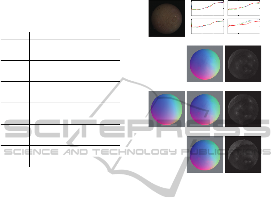
Table 2: The RMS errors of the estimated spectral re-
flectances of the color checker; the straightforward method,
our proposed method with the best set of light source, and
that with the worst set of light sources from top to bottom
in each field.
row\col.
1 2 3 4
0.054 0.080 0.044 N/A
1 0.059 0.078 0.043 N/A
0.060 0.078 0.044 N/A
0.051 0.075 0.060 0.015
2 0.072 0.070 0.107 0.016
0.070 0.070 0.101 0.015
0.040 0.049 0.123 0.025
3
0.039 0.057 0.109 0.025
0.039 0.055 0.110 0.024
0.044 0.060 0.088 0.059
4 0.041 0.065 0.080 0.057
0.039 0.063 0.081 0.059
0.068 0.061 0.048 0.063
5 0.081 0.058 0.042 0.070
0.081 0.058 0.041 0.069
0.025 0.068 0.037 0.038
6
0.030 0.067 0.027 0.052
0.030 0.067 0.027 0.050
by using the straightforward method and by using
our method with the best and the worst sets of light
sources from top to bottom in each field. The aver-
ages of the RMS errors are 0.056, 0.058, and 0.058
respectively. This result quantitatively demonstrates
that our method can accurately estimate spectral re-
flectances even from a small number of images.
Second, we evaluated the estimated surface nor-
mals. Figure 6 shows the image (a) and the es-
timated spectral reflectances (b) and normals of a
wooden ball. (d), (f), and (h) are the normals esti-
mated by using the straightforward method and our
proposed method with the best and the worst sets of
light sources. (e), (g), and (i) show the differences
between the ground truth (c) and the estimated ones
(d)(f)(h). We assume that the shape of the ball is a
perfect sphere although it looks a little distorted both
locally and globally to some extent. Therefore, a part
of the errors common to the estimated surfacenormals
by using the straightforward method and our method
would be due to those distortions. In addition, we
can observe white spots caused by specular reflection
components. The average errors of normals estimated
by using the straightforward method and our method
with the best and the worst sets of light sources are
5.11
◦
, 5.52
◦
, and 7.43
◦
respectively including the de-
viation of the ball from a perfect sphere and the errors
due to specular reflection components. Thus, we can
see quantitatively that our method can accurately es-
timate normals even from a small number of images.
(d) (e)
(f) (g)(c)
(h) (i)
(a) (b)
0
0.5
1
400 500 600 700
0
0.5
1
400 500 600 700
0
0.5
1
400 500 600 700
0
0.5
1
400 500 600 700
+
+
+
+
(i)
(ii)
(iii)
(iv)
(i) (ii)
(iii) (iv)
Figure 6: The estimated spectral reflectances (b) at four
points on the wooden ball (a). The red-solid lines, green-
dotted lines, and blue-dotted lines stand for the straightfor-
ward method and our proposed method with the best and
the worst set of light sources. (d), (f), and (h) are the nor-
mals estimated by using the straightforward method and our
method with the best and the worst sets of light sources. (e),
(g), and (i) show the differences between the ground truth
(c) and the estimated ones (d)(f)(h), and demonstrates that
our method performs as well as the straightforward method
when the best set of light sources is used.
6 APPLICATION
To demonstrate the effectiveness of estimating both
the spectral reflectances and normals by using our
proposed method, we synthesized images under novel
illumination conditions. Figure 7 shows the synthe-
sized images of the plaster relief and wooden ball un-
der 9 different illumination conditions; three spectral
distributions times three light source directions. The
spectral reflectances and normals estimated by using
the straightforward method (top) and our proposed
method (bottom) are used. We can see that the syn-
thesized images look quite natural, and that the bot-
tom images are consistent with the top images. This
result demonstrates that our proposed method extends
the capability of spectral relighting (Park et al., 2007;
SimultaneousEstimationofSpectralReflectanceandNormalfromaSmallNumberofImages
311

0
0.5
1
400 500 600 700
0
0.5
1
400 500 600 700
0
0.5
1
400 500 600 700
0
0.5
1
400 500 600 700
0
0.5
1
400 500 600 700
0
0.5
1
400 500 600 700
Figure 7: The synthesized images under novel illumination
conditions. The spectral reflectances and normals estimated
by using the straightforward method (top) and our proposed
method (bottom) are used.
Han et al., 2013) so that one can deal with novel
light source directions. Note that some artifacts due
to specular reflection components are observed on
the ball because our method assumes the Lambertian
model.
7 CONCLUSION AND FUTURE
WORK
In this study, by integrating multispectral imaging
and photometric stereo, we proposed a method for si-
multaneously estimating the spectral reflectance and
normal per pixel from a small number of images
taken under multispectral and multidirectional light
sources. In addition, taking attached shadows ob-
served on curved surfaces into consideration, we de-
rived the minimum number of images required for the
simultaneous estimation and proposed a method for
selecting the optimal light sources in terms of noise.
Through a number of experiments using real im-
ages, we showed that our proposed method can es-
timate spectral reflectances without the ambiguity of
per-pixel unknown scales, and that, when the opti-
mal set of light sources is used, our method using
only 9 images performs as well as the straightforward
method using a large number of images. In addition,
we demonstrated that estimating both the spectral re-
flectances and normals is useful for relighting under
novel light source spectral distributions as well as un-
der novel light source directions.
One direction of future study is the extension to
non-Lambertian surfaces. As mentioned in Section 5
and Section 6, the estimated spectral reflectances and
normals are sometimes contaminated by specular re-
flection components since we assume the Lambertian
model. We will use the robust estimation for remov-
ing those components as outliers or model them by
using parametric or non-parametric representation in
the future.
ACKNOWLEDGEMENTS
A part of this work was supported by JSPS KAK-
ENHI Grant No. 25280057.
REFERENCES
Ajdin, B., Finckh, M., Fuchs, C., Hanika, J., and
Lensch, H. (2012). Compressive higher-order sparse
and low-rank acquisition with a hyperspectral light
stage. Technical report, Eberhard Karls Universit¨at
T¨ubingen. WSI-2012-01.
Drbohlav, O. and Chantler, M. (2005). On optimal light
configurations in photometric stereo. In Proc. IEEE
ICCV2005, volume 2, pages 1707–1712.
Gat, N. (2000). Imaging spectroscopy using tunable filters:
a review. In Proc. SPIE Wavelet Applications VII, vol-
ume 4056, pages 50–64.
Gu, J. and Liu, C. (2012). Discriminative illumination:
per-pixel classification of raw materials based on op-
timal projections of spectral BRDF. In Proc. IEEE
CVPR2012, pages 797–804.
Han, S., Sato, I., Okabe, T., and Sato, Y. (2013). Fast spec-
tral reflectance recovery using DLP projector. IJCV.
DOI 10.1007/s11263-013-0687-z.
Okabe, T., Sato, I., and Sato, Y. (2009). Attached shadow
coding: estimating surface normals from shadows un-
der unknown reflectance and lighting conditions. In
Proc. IEEE ICCV2009, pages 1693–1700.
Park, J.-I., Lee, M.-H., Grossberg, M., and Nayar, S. (2007).
Multispectral imaging using multiplexed illumination.
In Proc. IEEE ICCV2007, pages 1–8.
Parkkinen, J., Hallikainen, J., and Jaaskelainen, T. (1989).
Characteristic spectra of munsell colors. JOSA A,
6(2):318–322.
Schechner, Y. and Nayar, S. (2002). Generalized mosaicing:
wide field of view multispectral imaging. IEEE Trans.
PAMI, 24(10):1334–1348.
Schechner, Y., Nayar, S., and Belhumeur, P. (2003). A
theory of multiplexed illumination. In Proc. IEEE
ICCV2003, pages 808–815.
Wellman, J. (1981). Multispectral mapper: imaging spec-
troscopy as applied to the mapping of earth resources.
In Proc. SPIE Imaging Spectroscopy, volume 268,
pages 64–73.
VISAPP2015-InternationalConferenceonComputerVisionTheoryandApplications
312

Woodham, R. (1980). Photometric method for determin-
ing surface orientation from multiple images. Optical
Engineering, 19(1):139–144.
Yamaguchi, M., Haneishi, H., Fukuda, H., Kishimoto, J.,
Kanazawa, H., Tsuchida, M., Iwama, R., and N, O.
(2006). High-fidelity video and still-image commu-
nication based on spectral information: natural vision
system and its applications. In Proc. SPIE-IS&T Elec-
tronic Imaging, volume 6062.
APPENDIX A
We give a counterexample and prove that 2 images (or
2 light sources) are insufficient for illuminating every
point on an arbitrary convex surface at least once. Let
us consider a unit sphere illuminated by a single direc-
tional light source. The single light source illuminates
at most almost the half of the occluding boundary of
the sphere according to the assumption of illuminated
pixels in eq.(12). Then, the length of illuminated oc-
cluding boundary is (π − δ), where δ is a small num-
ber. Since the length of the entire occluding bound-
ary is 2π and (π − δ) × 2 < 2π, we cannot illuminate
the entire occluding boundary at least once by using
2 light sources.
APPENDIX B
In a similar manner to Appendix A, we give a
counterexample and prove that 8 images (or 8 light
sources) are insufficient for illuminating every point
on an arbitrary convex surface at least 4 times, i.e. for
satisfying the condition (A) in subsection 4.3. Con-
sidering a unit sphere illuminated by a single direc-
tional light source, the length of illuminated occlud-
ing boundary is (π− δ). Since (π− δ)× 8 < 4×2π, it
is clear that we cannot illuminate the entire occluding
boundary at least 4 times by using 8 light sources.
SimultaneousEstimationofSpectralReflectanceandNormalfromaSmallNumberofImages
313