Second Degree of Freedom of Elastic Objects

Adjustable Poisson’s Ratio for Mass Spring Models

Maciej Kot and Hiroshi Nagahashi

Imaging Science and Engineering Laboratory, Information Processing Department,

Tokyo Institute of Technology, Tokyo, Japan

Keywords:

Mass Spring Models, Deformable Objects.

Abstract:

In this paper, we show how to construct mass spring models for the representation of homogeneous isotropic

elastic materials with adjustable Poisson’s ratio. Classical formulation of elasticity on mass spring models

leads to the result, that while materials with any value of Young’s modulus can be modeled reliably, only

ﬁxed value of Poisson’s ratio is possible. We show how to extend the conventional model to overcome this

limitation.

1 INTRODUCTION

Computer graphics community has been using mass

spring models (MSMs) for the representation of de-

formable objects since the earliest attempts to accom-

modate elastic solids in computer generated anima-

tions. While MSMs were popular because of their

low implantation complexity, the link between their

physical properties and spring-network parameters

has never been properly established. This led to be-

lief that MSMs cannot represent elastic objects accu-

rately and that the models do not converge to certain

solutions upon mesh reﬁnement (Van Gelder, 1998;

Nealen et al., 2006). Consequently more physically

accurate techniques such as ﬁnite element method

(FEM) gained popularity.

The accuracy of the description of an elastic object

is, however, not a problem in MSM representations.

The standard lattice based models used in physics,

mechanical engineering and other related ﬁelds of-

fer a description of elastic solids, which is as accu-

rate as the limitations of linear elasticity theory allow

it to be (Ladd and Kinney, 1997; Ostoja-Starzewski,

2002; Kot et al., 2014). There is however a limitation

to what can be modeled with MSMs. The classical

models allow to obtain any value of Young’s modu-

lus E, however Poisson’s ratio ν is limited to 1/4 for

volumetric objects and 1/3 for 2D meshes. This al-

lows to freely adjust the stiffness of an object, but is

not sufﬁcient to replicate all types of materials. In this

work we show how to efﬁciently extend conventional

MSM to overcomethis limitation and obtain a reliable

model of any homogeneous isotropic solid.

2 MASS SPRING MODELS

If we consider a homogeneous isotropic solid, its

elastic properties are deﬁned by exactly two param-

eters (elastic moduli). Classically Young’s modulus

E and Poisson’s ratio ν are the popular pair. The

Young’s modulus is the ratio of stress to strain mea-

sured along the same axis under an uniaxial stress

condition, that is, it gives the resistance to directional

stretching/compression. The Poisson’s ratio is the ra-

tio of transverse to axial strain (denotes to what de-

gree material expands in one direction when com-

pressed in another). Depending on the application,

besides E and ν, other moduli are often used such as

bulk modulus K, or Lam´e parameters λ and µ. In any

description only two of them are independentand pro-

viding a link between spring-network parameters, and

a chosen pair of the elastic moduli is sufﬁcient to de-

scribe elastic properties of the MSM.

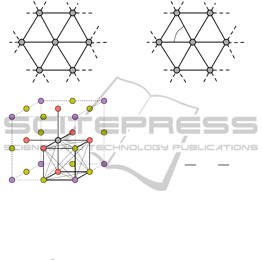
In case of 2D MSM, an isotropic homogeneous

structure can be obtained with hexagonal lattice

(Fig. 1) (Ostoja-Starzewski, 2002). All the springs

have the same spring coefﬁcient k and the relation be-

tween the spring coefﬁcient and the Lam´e constants

for a such network are given by

λ = µ =

√

k, (1)

from which it follows that E =

√

k and ν =

Springs are assumed to be of a unit length.

Similarly a volumetric isotropic solid can be con-

structed with cubic lattice MSM (Ladd and Kinney,

138

Kot M. and Nagahashi H..

Second Degree of Freedom of Elastic Objects - Adjustable Poisson’s Ratio for Mass Spring Models.

DOI: 10.5220/0005303601380142

In Proceedings of the 10th International Conference on Computer Graphics Theory and Applications (GRAPP-2015), pages 138-142

ISBN: 978-989-758-087-1

 2015 SCITEPRESS (Science and Technology Publications, Lda.)

Figure 1: Hexagonal lattice.

C B C

B A B

C B C

B A B

A A

B A B

C B C

B A B

C B C

Figure 2: Cubic lattice. The nearest neighbors of a node are

classiﬁed in three groups A, B and C. They correspond to

the potential connections along cube edges, face diagonals

and cube diagonals.

1997). The spring connections are present between

nearest neighbors (A) and second nearest neigh-

bors (B) (Fig. 2) and all have the same spring co-

efﬁcient k. The elastic moduli for such network are

given by

E = 2.5

ν = 1/4, (2)

where a is the length of an edge of an elemental

cube.

The models discussed above have a limitation on

the value of Poisson’s ratio, which comes from a well-

established result of the continuum mechanics. If

the constituents of a material interact with the cen-

tral forces dependent upon distance alone the Pois-

son’s ratio of a homogeneous and isotropic material is

identically 1/4 (or 1/3 for a 2D system) (Love, 1906;

Lakes, 1991). Other values of the Poisson’s ratio can

be obtained by incorporating non-central forces into

the model, e.g. the angular terms, or forces that do not

depend on distance alone or by introducinganisotropy

(Lakes, 1991).

Figure 3: Hexagonal lattice with normal as well as angular

springs.

An example of such extension is the Kirkwood

model of an isotropic 2D material (Ostoja-Starzewski,

2002). It is based on a hexagonal lattice and intro-

duces additional angular springs, which provide a re-

sisting force when an angle between two coinciding

springs changes from its neutral value of 60

◦

(Fig. 3).

The Poisson’s ratio is given by



1−

3β

2ka

.

3β

2ka



, (3)

where a is a length of an edge of a triangle, k is a

spring stiffness coefﬁcient of regular springs and β of

angular ones.

Similar modiﬁcations are possible in case of 3D

materials and the problem of constructing MSM-like

models capable of representing isotropic materials

with arbitrary values of Poisson’s ratio have been ex-

plored before by a number of researchers (Baudet

et al., 2007; Lakes, 1991; Zhao et al., 2011). An

overview of well established techniques can be found

in (Sahimi, 2003). Typically additional degrees of

freedom are added to the model by incorporating

beams, angular springs and other custom three or

four node connections which react not only to stretch-

ing, but shearing or applying toque as well. Intro-

ducing such elements allows to obtain wide range of

materials, however as volumetric objects are inher-

ently more complex than two dimensional structures,

the description of their properties tends to be more

complex as well. Analytical solutions are in most

cases too difﬁcult to derive and obtaining desirable

properties of such models often involves a numerical

minimization and parameter ﬁtting, which tunes the

model to the particular problem at hand. This fact,

together with increased computational and memory

costs, makes such models less suitable for practical

applications.

In contrast in this work we will explore an ap-

SecondDegreeofFreedomofElasticObjects-AdjustablePoisson'sRatioforMassSpringModels

139

Figure 4: Momentum ﬂow through a simple MSM.

proach of constructing MSM which allows to achieve

arbitrary values of ν, without introducing additional

structures into the model. Our approach will in fact

make use only of nodes and their relative pairwise dis-

tances.

3 EXTENDED MASS SPRING

MODELS

Simple MSMs described in Section 2 can be viewed

as a network in the Fig. 4. Forces in such networks

act along straight lines between particles, and as we

know, this leads to ν = 1/4, which may be considered

a geometric property of the space (the way distance

to neighboring nodes changes, when we change the

position of a node).

We generalize this model by introducing addi-

tional phenomenon. When two nodes approach, they

start repelling each other as usual, and additionally

each of them starts radiating momentum in ”random”

directions.

To visualize how we can justify such behavior,

let us consider a particle-carrier interaction model in

which we assume, that constituents of the matter (par-

ticles) interact with each other by means of exchang-

ing carriers (which in turn can be considered a small

particles). Carriers interact with particles (and with

each other) by means of central forces (elastic colli-

sions), therefore this model still uses central forces

as most basic means of interaction. Carriers how-

ever have a ﬁnite velocity so the transfer of momen-

tum does not happen instantaneously; the big particles

move as well. Having this in mind, we may assume

that a carrier shot form one particle, may not hit the

other particle with a sniper’s precision. In such case

it will disperse in a ”random” direction and will not

Figure 5: Dispersive momentum ﬂow.

Figure 6: Momentum dispersion.

come back to the ﬁrst particle (Fig. 6). If a particle

is bombarded from all directions uniformly, the dis-

persed carriers will also appear to be radiating from

the particle uniformly (even if the actual distribution

of dispersion angles is not trivial).

Figure 5 illustrates the dissipative part of the inter-

action, where each node absorbs the incoming carri-

ers and radiates them uniformly in all directions. Such

network will behave like a gas or ﬂuid with no viscos-

ity.

We will model this phenomenon using MSMs in

the following way. When two nodes approach each

other causing increase of momentum ﬂow between

them, only a fraction of the ﬂow will participate in

the direct exchange of momentum between these two

nodes and appear as a regular force of the spring

= −κ

∆L. The rest of the ﬂow will be distributed

uniformly to all springs connected to a node (scaled

to the length of a spring), causing dissipation of mo-

mentum F

∗

= −qκ

∆L. Parameter q denotes the ratio

between dissipative momentum ﬂow, and the direct

one.

Material modeled in such way is now character-

ized by two parameters – µ gives the strength of direct

interactions, and q[µ] of the dispersive ones.

The standard expression for a stress in an elastic

body

= Kδ

+ 2µ(ε

−

), (4)

can be rewritten, by treating our material as a su-

perposition of Cauchy’s isotropic structure, in which

GRAPP2015-InternationalConferenceonComputerGraphicsTheoryandApplications

140

λ = µ with a ﬂuid in which σ

= Bε

, where Bε

corresponds to pressure.

= µδ

+ 2µε

+ Bδ

, B = λ−µ (5)

µδ

+ 2µ(ε

−

) + Bδ

(6)

The direct interactions will correspond to µ pa-

rameter, dispersive ones to B. Both can be controlled,

which allows to achieve other values of Poisson’s ra-

tio:

ν =

B+ µ

2(B+ 2µ)

, (7)

ν =

2(2+

, Q =

, (8)

where in a perfect structure Q = 2q, and it denotes

the ratio between dispersed and not dispersed carriers.

The multiplication by the factor of 2 is introduced for

convenience (one spring connects two nodes).

4 TESTS

We have applied our technique to Ladd’s cubic lat-

tice models and veriﬁed that we are able to obtain any

value of Poisson’s ratio with their use.

In order to estimate numerically the values of E

and ν in an MSM, the following numerical experi-

ment has been performed: a block of an elastic mate-

rial was compressed by applying static displacement

to its opposite ends along x direction, and the resulting

deformation was measured both for random and cubic

MSMs. The Young’s modulus and Poisson’s ratio are

related to the elastic response of such a system by

E =

F/A

∆x/L

ν =

∆y

∆x

where F is the reaction force, A the cross-sectional

area of the block (in YZ plane), and ∆x and ∆y are

the deformations of the block along x and y direc-

tions respectively. The initial block dimensions were

70a

×15a

(where a

is an arbitrary unit of

length) and the base spring constant has been set to k

The static displacement in x direction was imposed on

all the nodes on the boundary of the block.

The results are presented in Fig. 7 and they con-

ﬁrm that any value of Poisson’s ratio can be achieved

with a very high accuracy. Figure 8 shows visual ex-

amples of a few chosen materials with different ν. Al-

though the presented shapes are very simple, the tests

-1.2

-1

-0.8

-0.6

-0.4

-0.2

0.2

0.4

0.6

-1 -0.5 0 0.5 1 1.5 2 2.5 3

Poisson’s ratio

Figure 7: Poisson’s ratio in Cubic lattice MSM. Red curve

represents a theoretical prediction. Blue points are the re-

sults of measurements.

show that our extended MSM is capable of modeling

bulk materials accurately. Given sufﬁciently high res-

olution any complex shape can be modeled reliably.

5 CONCLUSIONS

In this article we showed an approach of construct-

ing MSM which allows to achieve arbitrary values

of ν, without introducing additional structures into

the MSM. We demonstrated that by incorporating the

concept of momentum dispersion additional degree of

freedom can be added to the classical MSM, allowing

it to freely represent homogeneous isotropic materials

characterized by two different constants (in contrast

to one constant description given by classical MSM).

Because our method does not introduce additional el-

ements to the MSM itself, the memory costs remain

unchanged and the computational costs rise by much

lower degree when compared with methods which do

introduce additional elements to the MSM.

This makes our method useful for real time ap-

plications involving deformable elastic objects of any

kind (e.g. in computer games), and especially attrac-

tive for simulating fracture or crack propagation(peri-

dynamics) – the application for which MSMs are gen-

erally considered to be better suited than FEM based

approaches, but suffer from the fact that they cannot

represent all types of materials.

The simplest implementation of our model, when

used with explicit time integrator, requires additional

iteration through all the springs in the system, effec-

tively doubling the computational time when com-

pared to the simple MSM. Some improvements are

however possible; for instance the value of momen-

tum dispersed on the nodes in the ’previous’ frame

could be used to approximate the value in the current

frame, which eliminates the need of additional itera-

tion through the springs, but may inﬂuence the stabil-

ity of the simulation. However, in case of quasi-static

SecondDegreeofFreedomofElasticObjects-AdjustablePoisson'sRatioforMassSpringModels

141

Figure 8: A block of material with dimensions 2×3 ×2 compressed in y direction to 75% of its natural length. Different

values of Poisson’s ratio, from the left: -1, 0, 0.25, 0.47.

simulation (such as point based integration techniques

(Bender et al., 2013)), it should not affect the stability.

Additionally the accuracy of our models is ex-

pected to be higher than that of techniques involving

parameter ﬁtting and the analytical description of our

model is provided. This makes our MSM an attractive

starting point for developing more advanced models

(e.g. for anisotropic materials). In our model we have

assumed that the dispersion of the force happens uni-

formly in all directions. In MSMs it will translate into

equal redistribution of the incoming force to all the

springs connected with a node (scaled by the length).

Because redistribution is isotropic, so will be the elas-

tic properties of the material. However by introduc-

ing non uniform dispersion mechanisms it should be

possible to achieve non isotropic behaviors without

extensive modiﬁcations of the current model. Such

modiﬁcations may be a good direction for the future

work, as they would allow to efﬁciently model or-

ganic tissues e.g. for surgical simulations, the applica-

tion for which MSMs are still actively used, but once

again suffer from the lack of a mathematical model

that would allow to express their elastic properties.

ACKNOWLEDGEMENTS

Authors acknowledge the support of JSPS KAKENHI

(Grant Number 24300035).

REFERENCES

Baudet, V., Beuve, M., Jaillet, F., Shariat, B., and

Zara, F. (2007). Integrating Tensile Parameters in

3D Mass-Spring System. Technical Report RR-

LIRIS-2007-004, LIRIS UMR 5205 CNRS/INSA de

Lyon/Universit´e Claude Bernard Lyon 1/Universit´e

Lumi´ere Lyon 2/

Ecole Centrale de Lyon.

Bender, J., M¨uller, M., Otaduy, M. A., and Teschner, M.

(2013). Position-based methods for the simulation of

solid objects in computer graphics. In EUROGRAPH-

ICS 2013 State of the Art Reports. Eurographics As-

sociation.

Kot, M., Nagahashi, H., and Szymczak, P. (2014). Elas-

tic moduli of simple mass spring models. The Visual

Computer.

Ladd, A. J. C. and Kinney, J. H. (1997). Elastic constants

of cellular structures. Physica A: Statistical and The-

oretical Physics, 240(1-2):349–360.

Lakes, R. S. (1991). Deformation mechanisms in negative

Poisson’s ratio materials: structural aspects. Journal

of Materials Science, 26:2287–2292.

Love, A. E. H. (1906). A treatise on the mathematical the-

ory of elasticity. Cambridge University Press.

Nealen, A., M¨uller, M., Keiser, R., Boxerman, E., Carl-

son, M., and Ageia, N. (2006). Physically based

deformable models in computer graphics. Comput.

Graph. Forum, 25(4):809–836.

Ostoja-Starzewski, M. (2002). Lattice models in microme-

chanics. Applied Mechanics Reviews, 55(1):35–60.

Sahimi, M. (2003). Rigidity and Elastic Properties: The

Discrete Approach. Heterogeneous Materials: Linear

Transport and Optical Properties. Interdisciplinary

Applied Mathematics v 1, (Chapter 8). Springer-

Verlag New York.

Van Gelder, A. (1998). Approximate simulation of elastic

membranes by triangulated spring meshes. J. Graph.

Tools, 3(2):21–42.

Zhao, G.-F., Fang, J., and Zhao, J. (2011). A 3d distinct

lattice spring model for elasticity and dynamic fail-

ure. International Journal for Numerical and Analyt-

ical Methods in Geomechanics, 35(8):859–885.

GRAPP2015-InternationalConferenceonComputerGraphicsTheoryandApplications

142