Optimal Surface Normal from Afﬁne Transformation

Barath Daniel

1,2

, Jozsef Molnar

and Levente Hajder

1,2

Geometric Modelling and Computer Vision Laboratory, MTA SZTAKI, H-1111 Kende utca 13-17, Budapest, Hungary

Department of Image Processing and Computer Graphics, Institute of Informatics,

University of Szeged,

Arp

ad t

er 2., H-6720 Szeged, Hungary

Keywords:

3D Reconstruction, Normal Estimation, Calibrated Stereo Images.

Abstract:

This paper deals with surface normal estimation from calibrated stereo images. We show here how the afﬁne

transformation between two projections deﬁnes the surface normal of a 3D planar patch. We give a formula

that describes the relationship of surface normals, camera projections, and afﬁne transformations. This formula

is general since it works for every kind of cameras. We propose novel methods for estimating the normal of

a surface patch if the afﬁne transformation is known between two perspective images. We show here that the

normal vector can be optimally estimated if the projective depth of the patch is known. Other non-optimal

methods are also introduced for the problem. The proposed methods are tested both on synthesized data and

images of real-world 3D objects.

1 INTRODUCTION

Although computer vision has been an intensively

researched area in computer science from many

decades, several unsolved problems exist in the ﬁeld.

This paper proposes a novel optimal method for es-

timating the normal vector of a planar surface patch

if the afﬁne transformation of the patch between two

calibrated (stereo) images is known.

The normal vector estimation problem itself can

most accurately be solved by photometric stereo (PS)

that was introduced many decades ago (Woodham,

1978). The main drawback of this method is that it

can only be used in laboratories where light condi-

tions are totally controlled. PS usually assumes that

the object to be reconstructed is illuminated by di-

rectional light source(s) (Woodham, 1978), but point-

light sources can also be applied. (Fodor et al., 2014).

The image-based normal vector estimation is usu-

ally carried out by decomposing the homography of

the tangent plane between stereo images (Faugeras

and Lustman, 1988; Malis and Vargas, 2007). Unfor-

tunately, these methods ambiguous as it was shown in

several studies (e.g. in (Liu, 2012)). To the best of

our knowledge, the problem of image-based normal

vector estimation from afﬁne transformation has not

been solved yet. The ﬁrst similar work was published

in two papers by Habbecke and Kobbelt in (Habbecke

and Kobbelt, 2006; Habbecke and Kobbelt, 2007).

They estimate the parameters of a ﬂat patch based on

photo-consistency. The plane is parameterized in 3D

by the implicit parameters of a general plane. (These

are three real values as the implicit parameters of a

3D plane are deﬁned up to an arbitrary scale.) Our

method only concentrates on the estimation of the

spatial normal vector since the point of the plane can

be estimated in 3D by triangulation if corresponding

projections on two patches are known (Hartley and

Sturm, 1997; Hartley and Zisserman, 2003).

The closest work to our study is that of Megyesi

et al. (Z. Megyesi and D.Chetverikov, 2006). They

compute a dense 3D reconstruction using normal vec-

tors. The normal vectors themselves are calculated

from the afﬁne parameters between a rectiﬁed stereo

image pair. For this reason, only two parameters of

the afﬁne transformation have to be estimated. The

drawback of this work is that the rectiﬁcation itself

cannot be perfect due to noise and computational in-

accuracy. Our method proposing here is more general

as it works on arbitrary stereo image pairs. The only

restriction is that the stereo images have to be taken

by perspective cameras. (Or the non-perspective dis-

tortion of the images has to be undistorted.)

To the best of our knowledge, this is the ﬁrst

study that deals with surface normal computation

from afﬁne transformation using calibrated stereo im-

ages. The main contribution of this paper is twofold:

(i) We show here the general relationship among sur-

305

Daniel B., Molnar J. and Hajder L..

Optimal Surface Normal from Afﬁne Transformation.

DOI: 10.5220/0005303703050316

In Proceedings of the 10th International Conference on Computer Vision Theory and Applications (VISAPP-2015), pages 305-316

ISBN: 978-989-758-091-8

 2015 SCITEPRESS (Science and Technology Publications, Lda.)

face normal vector, afﬁne transformation and cam-

era parameters. The formulas proposing here is valid

for every kind of cameras. (ii) Different surface nor-

mal estimators are proposed here including an opti-

mal one that ﬁnds the optimal normal vector in the

least squares sense if the afﬁne parameters are con-

taminated with noise.

2 GEOMETRIC BACKGROUND

Two projections of a 3D surface are given in stereo

images. If the neighboring pixels are selected around

image locations, these pixels form the so-called

patches. The afﬁne transformation between two cor-

responding patches are assumed to be known. The

goal of this study is to show how the surface normal

n can be estimated if the images are calibrated. The

problem is visualized in Figure 1.

Figure 1: 3D patch perspectively projected to stereo images.

x = Π

(X,Y,Z) y = Π

(X,Y,Z)

The surface point [X ,Y,Z]

is written in parametric

form

X = X (u,v), Y = Y (u,v), Z = Z(u, v).

As it is well-known in differential geome-

try (Kreyszig, 1991), the tangent vectors of the

plane are written by the partial derivatives of the

spatial coordinates, while the surface normal is given

by the cross product of the tangent vectors.







∂X(u,v)

∂u

∂Y (u,v)

∂u

∂Z(u,v)

∂u













∂X(u,v)

∂v

∂Y (u,v)

∂v

∂Z(u,v)

∂v







n = S

× S

It is known that the 3D point [X,Y,Z]

, and tangent

vectors S

and S

determine the tangent plane. Lo-

cally, the surface can be approximated by its tangent

plane. We assumed that we have images taken from

the object. Now, a point of the surface close to the

given 3D location [X,Y,Z]

is approximated by the

ﬁrst order Taylor-series:



x + ∆x

y + ∆y



≈



(X,Y,Z)



∂Π

(X,Y,Z)

∂u

∂Π

(X,Y,Z)

∂v

∂Π

(X,Y,Z)

∂u

∂Π

(X,Y,Z)

∂v



∆u

∆v



Let us see that the partial derivatives of the projec-

tion functions give the afﬁne transformation between

3D and 2D surface patches.



∆x

∆y



≈ A



∆u

∆v



A =

∂Π

(X,Y,Z)

∂u

∂Π

(X,Y,Z)

∂v

∂Π

(X,Y,Z)

∂u

∂Π

(X,Y,Z)

∂v

The partial derivatives can be reformulated using the

chain rule. For instance,

∂Π

(X,Y,Z)

∂u

∂Π

(X,Y,Z)

∂X

∂u

∂Π

(X,Y,Z)

∂Y

∂u

∂Π

(X,Y,Z)

∂Z

∂u

= ∇Π

where ∇Π

is the gradient vector of the projection

function w.r.t. the spatial coordinates X, Y , and Z of

the surface patch. Similarly,

∂Π

∂v

= ∇Π

∂Π

∂u

= ∇Π

∂Π

∂v

= ∇Π

Therefore, the afﬁne matrix can be written as

A =



∇Π







In stereo vision, two images are given. The afﬁne

transformation between the image patches is obtained

by concatenating the inverse of afﬁne transformation

(between the patches of image #1 and the spatial

patch), and the afﬁne transformation A

(between 3D

patch and that in image #2). Formally, it can be writ-

ten as



∆x

∆y



= A

−1



∆x

∆y



VISAPP2015-InternationalConferenceonComputerVisionTheoryandApplications

306

−1

is the afﬁne transformation between the im-

ages. The inverse of the afﬁne matrix A can be written

−1

det (A)



−Π



where det(A) = Π

− Π

. If one

makes elementary modiﬁcation utilizing the fact that

− S

= [N]

, then the afﬁne transformation

−1

can be written as

−1

[N]

Note that the scale of the normal is arbitrary since

both the determinant and the matrix elements are mul-

tiplied with the scale of [N]

The expression a

[N]

b is also called the scalar

triple product. Remark that a

[n]

b equals to n

(b ×

a). Therefore, the ﬁnal equation of the afﬁne transfor-

mation is written as





= A

−1





(1)

where w

= ∇Π

× ∇Π

, w

= ∇Π

× ∇Π

, w

∇Π

× ∇Π

, w

= ∇Π

× ∇Π

, and w

= ∇Π

∇Π

. Equation 1 is a very important formula which

shows the relations of the surface normal and the pro-

jection of the surface to the stereo image pair. A very

important advantage of this formula is that it is valid

for every kind of camera since only the two projec-

tive equations must be known. We show here that

the above formula can be used to compute the surface

normal if the perspective parameters are calibrated.

2.1 Pin-hole Camera Model

When the standard perspective camera model is used,

the projection is written as

[x,y,1]

persp

[X,Y,Z, 1]

, (2)

where [x, y] are the projected coordinates in image

space, s is the projective depth, P

persp

is the so called

projection matrix with size 3 × 4. Let us denote the

rows of the projective matrix by p

, p

, and p

. The

projection formulas and their gradients can be written

[X,Y,Z,1]

∇Π





+ xP





∇Π





+ yP





where P

i j

is the element in the i

row and j

column

in projection matrix P

persp

. The projective depth is

obtained as s = p

[X,Y,Z, 1]

. The afﬁne transfor-

mation becomes





αn





(3)

where α = s

is the ratio of the projec-

tive depths in the ﬁrst and second images, and

= s



∇Π

× ∇Π



, w

= s



∇Π

× ∇Π



= s



∇Π

× ∇Π



, w

= s



∇Π

× ∇Π



and w

= s



∇Π

× ∇Π



A very important remark is that if the projective

depth s

is unknown, but the upper left 3 × 3 subma-

trices of the projection matrices P

and P

are known

then the gradient vectors can be calculated up to an

unknown scale. (This scale is the multiplicative in-

verse of the projective depth s

.) Also note that the

vectors w

.. .w

are scaled by s

while w

by s

Therefore, the normal vector is independent of the

translation between the two cameras since the last

columns of the projection matrices are the product

of the camera intrinsic parameters and the translation.

For this reason, the following two cases must be dis-

tinguished:

1. Both projection matrixes P

and P

are known.

(In other words, the cameras are calibrated.)

2. Only the upper-left 3 × 3 submatrices of the pro-

jections are known. In this case, the projective

depth of the points is not known. However, the

gradients can be computed up to a scale where this

scale is the inverse of the projective depth.

Also remark that the normal vector cannot be es-

timated if w

= 0. This can only be true if ∇Π

and

∇Π

are parallel which is not a realistic case as it is

only possible if the ﬁrst and second rows of the 3 × 3

submatrix of projection matrix P

persp

are parallel. If

the camera calibration is valid it cannot be true. The

problem itself is numerically stable if the angles be-

tween the vectors w

.. .w

are relatively large. To

our experiments, this is true for realistic reconstruc-

tion problems.

OptimalSurfaceNormalfromAffineTransformation

307

3 NORMAL VECTOR

ESTIMATION

This section shows different normal vector estimators.

The ﬁrst one is very fast and simple, later more so-

phisticated and accurate methods are introduced.

3.1 Fast Normal Estimation (FNE)

The base matrix equation (Eq. 3) consists of 4 ele-

ments. If two of those are selected and they are di-

vided by each other, then an equation is obtained. If

the same procedure is repeated for the rest of the ma-

trix elements, then the second equation can be simi-

larly yielded. For instance, two elements of the ﬁrst

and second rows give the equations

(4)

(5)

These equations can be trivially modiﬁed as



− a



n = 0



− a



n = 0

The normal vector n is perpendicular to both a

−

and a

−a

. Therefore, the normal can be

obtained as the cross product of these vectors:

n =



− a





− a



. (6)

Of course, the obtained vector n should be normal-

ized, its length must be 1. A very nice property of

this normal estimation is that it is independent of the

scales appearing in vectors w

.. .w

. Therefore, the

projective depths of the patch are not required to es-

timate the normal, because they inﬂuence only the

length of n.

Remark, that the equation pairs (Eq. 4 & 5) can be

selected in other two ways. In those cases, the normal

vector is given by

n =



− a





− a



(7)

n =



− a





− a



(8)

3.2 Optimal Normal Estimation with

Known Projective Depth (OPT)

The aim of the optimal method is to minimize the er-

ror in the matrix base equation (Eq. 3). Formally, the

estimation itself can be written as the minimization of

Frobenius norm of Equation 3 with respect to normal

n. This is equivalent to

argmin

∑

k=1



− a



(9)

It minimizes the normal vector in the least square

sense assuming that the afﬁne parameters are contam-

inated with noise. (This assumption is valid since the

afﬁne parameters are estimated as described later in

Sec. 4.2 in short, and this estimation cannot be per-

fect since the images themselves contain noise.) The

optimal solution is given in ﬁrst part of the Appendix

with α = 1.

3.3 Normal Estimation with Unknown

Projective Depths using Alternation

(ALT)

If the projective depth is unknown then the base opti-

mization equation (Eq. 9) cannot be applied since the

parameter α = s

is not known. The cost function

deﬁned in Eq. 9 has to be modiﬁed as

argmin

∑

k=1



αn

− a



(10)

Unfortunately, this problem cannot be optimally

solved to the best of our knowledge. We propose here

an alternating-like approach which is overviewed in

Alg. 1. The alternation has two steps:

1. EstimateAlpha: The cost function (Eq. 10) is a

linear one with respect to 1/α since it can be

written as A

= b where A =

,. ..,

and b = [a

,. .., a

]

. The optimal solution of an

overdetermined linear system can be solved opti-

mally. In this case, that is obtained as

∑

)

∑

(11)

2. EstimateNormal: The normal vector estimation

is very similar to the optimal method described

above, the only difference is that the parameter

α appears in the denominators. However, the

method described in Appendix can solve the sub-

problem optimally.

The alternation requires initial values for the parame-

ters n and α to be optimized. We propose to use the

linear methods described later in Sec 3.4.2 in order to

compute the initial values. The alternation converges

to the closest (local) minimum since it optimizes a

non-negative cost function and each step decreases

(or does not increase) the cost. Unfortunately, we

VISAPP2015-InternationalConferenceonComputerVisionTheoryandApplications

308

could not prove theoretically that the global optimum

is reached in this way, however, to our practice, the

method usually improves the initial normal n.

Algorithm 1 : Alternation for Normal Estimation

(ALT).

n, α ← Parameter Initialization by LNE-UPD

repeat

α ← EstimateAlpha(n,w

,. .., w

)

n ← EstimateNormal(α,w

,. .., w

)

until convergence

3.4 Linear Normal Estimation (LNE)

The base matrix equation (Eq. 3) is a nonlinear one.

The elements can be linearized if they are multiplied

with their common denominator αw

n. Then a cost

function can be formed for the elements as

argmin

∑

k=1



− αa



(12)

This is a usual trick, and the solution will not be op-

timal if this modiﬁcation is carried out. However,

the problem becomes linear, and it can be solved eas-

ily (Bj

orck, 1996).

3.4.1 Linear Normal Estimation for Known

Projective Depth (LNE-KPD)

If the projective depth is known, then α = 1 and the

problem can be rewritten as an overdetermined ho-

mogenous linear equation system An = 0 subject to

n = 1, where

A =







− a







(13)

The optimal solution of this system is the eigenvector

of matrix A

A corresponding to the smallest eigen-

value (Bj

orck, 1996).

3.4.2 Linear Normal Estimation for Unknown

Projective Depth (LNE-UPD)

If the projective depth is unknown, then the function

to be optimized in Eq. 12 gives an overdetermined ho-

mogenous linear system Bb = 0, similarly to the pre-

vious case (Sec. 3.4.1), but the matrix of coefﬁcients

B and the vector b differ as follows.







, −a







b =



αw



The solution is given from the eigenvector of

matrix B

B corresponding to the smallest eigen-

value (Bj

orck, 1996). If this vector is denoted by

then the estimation for the normal vector n is given by

the ﬁrst three coordinates of

b, but this vector should

be normalized in order to fulﬁll the n

n = 1 con-

straint. The parameter α = s

can also be com-

puted if n is known from the fourth coordinate of

4 EXPERIMENTAL RESULTS

The proposed normal vector estimators have been

tested both on synthesized data and real world images.

4.1 Test on Synthesized Data

During synthesized tests, our main goal was to gener-

ate different normal vectors with corresponding afﬁne

parameters. For this reason, a stereo image pair was

ﬁrst generated represented by their 3 × 4 projection

matrices. Then a 3D sphere was generated as well

sampled by spherical coordinates. The normal vector

of the locations on the sphere can easily be calculated

as it is the direction pointing from the sphere center to

the current surface points. The synthetic sphere with

the ground truth normals is visualized in Fig. 2. 72

different patches sampled by spherical coordinates are

used in order to compare the methods.

Figure 2: Sphere with normal vectors for synthesized test.

The afﬁne parameters between the stereo images

were calculated as follows: (i) The tangent plane of

the sphere was determined ﬁrst, (ii) then it was pro-

jected to the stereo images. (iii) The projections of

OptimalSurfaceNormalfromAffineTransformation

309

the plane determine two homographies with respect to

the 3D tangent plane. (iv) The homography between

the two images were given by concatenating the two

3D→2D homographies. (v) The afﬁne transforma-

tion is the ﬁrst order approximation of the 2D→2D

homography at the given locations.

The error values are deﬁned as the average of the

angle error between the estimated and ground truth

normal vectors. We have tested all the methods de-

scribed in this study. In each test case, 72 patches of

the sphere were generated, and the tests were repeated

50 times. Thus, the average error values come from

72 · 50 = 3600 run of the competitor methods. Two

test cases were simulated: zero-mean Gaussian noise

was added to the (i) afﬁne parameters and (ii) to the

elements of the projection matrices.

Remark that all the synthesized tests have been

implemented on Octave

4.1.1 Test with Contaminated Afﬁne Parameters

We have compared the efﬁciency of the fast (FNE),

alternation (ALT) and optimal (OPT) normal estima-

tors. It is clear that the optimal estimator (OPT) out-

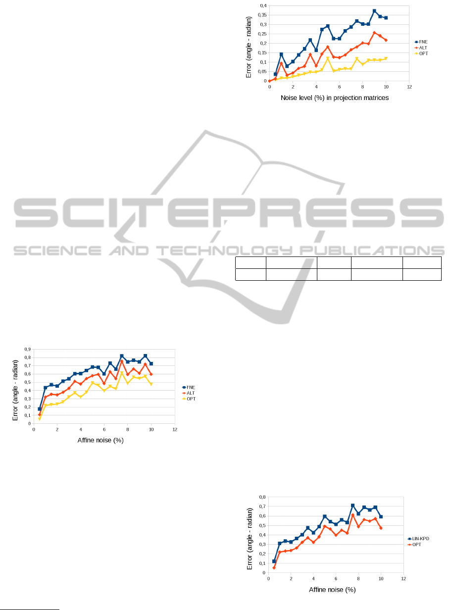
performs the others as it is visualized in Fig. 3 since

it optimally estimates the normal vector in the least

square sense. It is also obvious that the fast method is

the less accurate one as the other two methods (OPT

and ALT) are signiﬁcantly more sophisticated.

Figure 3: Comparison of methods when afﬁne parameters

contaminated.

We have also compared the linear methods to the

corresponding non-linear ones. Namely, the linear

method with unknown projective depth (LIN-UPD)

algorithm is compared to the alternation (Fig. 5) and

linear with known projective depth method (LIN-

KPD) to the optimal one ((Fig. 6)). The differences

are signiﬁcant only if the optimal (OPT) method is

used instead of its linear version.

We have also examined the expected values and

the spreads of the ﬁve proposed methods. The ex-

pected value for the length of the difference between

www.octave.org.

Figure 4: Comparison of methods when projective parame-

ters contaminated.

the ground truth and estimated vectors are close to

zero as it is excepted. Therefore, the estimators are

consistent. Their spreads are listed in Table 1. It

shows that the optimal method has the lowest spread

as it is expected, FNE is the highest one. It is inter-

esting that the linear method with known projective

depths gives signiﬁcantly better result than the meth-

ods with unknown depths (LIN-UPD and ALT),

Table 1: Spread of error vector lengths.

FNE LIN-UPD ALT LIN-KPD OPT

0.55 0.449 0.433 0.352 0.2919

4.1.2 Test with Contaminated Projection

Parameters

Another interesting experiment is when the elements

of the projection matrices are contaminated with

noise. We have examined the same test cases as

in Sec.4.1.1.

When the base FNE, ALT and OPT methods

are compared, the dominance of the optimal method

(OPT) is more obvious. The performance of the fast

(FNE) and alternation (ALT) methods are closer to

each other than in the previous test case (Sec. 4.1.1).

The accuracy of the result is also the best (highest) for

the optimal method. It seems that the other two meth-

ods (FNE and ALT) are very sensitive to noise since

the corresponding charts (Fig. 4) contain many peaks.

Figure 5: Comparison of linear and corresponding nonlin-

ear methods.

VISAPP2015-InternationalConferenceonComputerVisionTheoryandApplications

310

Figure 7: Comparison of normal vector estimators. HOM: normal from homography decomposition AFF: normal from afﬁne

parameters by proposed OPT method. Left: transformation estimated from 4 points, Center: 6 points, Right: 8 points.

Figure 6: Comparison of linear and corresponding nonlin-

ear methods.

To conclude this synthetic test, it can be declared

that the optimal method is the best solution if the pro-

jective depth of the 3D point is known. If it is not, the

alternation method serves the most efﬁcient method,

but its advantage over its linear version is very small.

The alternation itself is an iterative algorithm, some-

times it can be very slow. Therefore, we propose the

LIN-UPD method for time-critical application, ALT

is the best selection for ofﬂine algorithms when the

projective depths are unknown.

4.1.3 Normal Vector from Afﬁne Parameters

Versus Homography

The mainstream solution for computing the normal

vector from two patches is to estimate the homogra-

phy between the patches (Malis and Vargas, 2007).

It has eight degrees of freedom, and it can be decom-

posed into the pose (3 DoF), the location (3 DoF), and

the normal (2 DoF) of the plane.

We compare the accuracy of the homography-

estimated normal vector with our optimal (OPT) esti-

mator. The synthesized data is given by sampling the

surface of a sphere similarly to the synthesized tests

above. However, the homography and the afﬁne trans-

formation are both estimated from projected points:

points are generated randomly on the 3D tangent

plane (close to the location on sphere surface), and

these points are projected to the image pair. Then

noise is added to the projected coordinates in image

space. The homography and the afﬁne transformation

are estimated using the corresponding points in im-

age pairs. The estimation of the afﬁne transformation

is easier since it is trivial that afﬁne parameter esti-

mation is a linear problem. We estimate the homogra-

phy via numerical optimization method, the initial pa-

rameters are computed by DLT (Direct Linear Trans-

formation) algorithm (Hartley and Zisserman, 2003).

Note that at least 4 points are required to estimate the

homography, while 3 points are sufﬁcient to compute

the afﬁne transformation.

The results of the comparison is visualized in

Fig. 7. The transformations are estimated from the

same point correspondences. The number of cor-

responding points are 4, 6, and 8 as it is seen in

Fig. 7. The methods are denoted by ’HOM‘ (nor-

mals from estimated homography) and ’AFF‘ (nor-

mals from afﬁne transformation). It is interesting that

AFF serves better results when the noise is low. It is

true especially for the P = 4 case (left image in Fig. 7).

It is because the homography is determined exactly by

the given 4 points, while the afﬁne transformation is

overdetermined. When the number of points grows

(center and right plots on Fig. 7), the normal from ho-

mography estimation becomes better than that from

afﬁne transformation since the projected coordinates

are obtained via perspective projection, and homog-

raphy represents the correct transformation between

corresponding planes in image space.

4.2 Test on Real Image Pairs

Real Tests on Calibrated Images. The proposed op-

timal normal estimator has been also tested on real

data. In order to use the normal estimator, the projec-

tion matrices have to be known. We have downloaded

building images and reconstruction data with camera

parameters from the web page of the Visual Geometry

Group at Oxford University

The Oxford data sets contain point correspon-

dences, but we have used ASIFT method (Yu and

Morel, 2011) of Yu et al. for this purpose instead of

using the original data. The afﬁne transformations for

the pairs are computed as follows. (1) Two patches

around the corresponding locations are cropped from

http://www.robots.ox.ac.uk/ vgg/data/

OptimalSurfaceNormalfromAffineTransformation

311

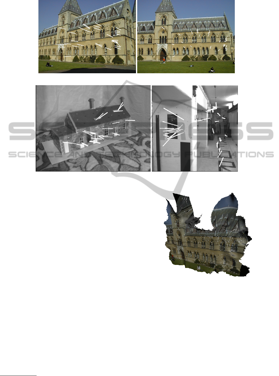
Figure 8: Stereo image pair with estimated normals (Library sequence).

Figure 10: Estimated normals on sequence House (left) and Corridor (right).

the images. Their size are from 60 × 60 to 80 × 80

depending on test sequences. (2) Then the ASIFT

method (Yu and Morel, 2011) is applied again for the

patch pair obtaining point correspondences between

patches. Estimating the afﬁne transformation is

an afﬁne 2D registration problem based on point

correspondences. It is easy to solve since the problem

is linear w.r.t. afﬁne parameters, the parameters can

be obtained optimally (Bj

orck, 1996) even if the

problem is overdetermined. Remark that the afﬁne

estimator should be robust since ASIFT can give false

correspondences. We used a RANSAC (Fischler and

Bolles, 1981)-like algorithm to discard the outliers.

The proposed optimal method is carried out on the

computed afﬁne transformations of the Library,

House, and Corridor pairs as it is seen in Figs. 8.

10. The normals are visualized by white rods. It is

evident that the quality of a normal depends on the

baseline of the stereo images. The last stereo pair

(Corridor) has shorter baseline than the other two,

the accuracy of its estimated normals (on the ﬂoor

and wall) are lower.

We were able to reconstruct the 3D surface of the

estimated positions and corresponding normals using

the Marching Cubes (APSS) ﬁlter of MeshLab

. It is

visualized in Fig 9.

www.meshlab.org

Figure 9: Reconstructed 3D model.

Normal from Real Planar Surfaces. The proposed

normal vector estimator (OPT) is also tested on im-

ages of buildings as it is pictured in Fig 11. These

objects mainly consist of planar walls and they can be

matched by homography-based pairing methods es-

pecially when the images are rectiﬁed (Tanacs et al.,

2014). Thought the homography itself can be de-

composed (Faugeras and Lustman, 1988) if the cam-

eras are calibrated, and then the plane normal is ob-

tained with the camera extrinsic parameters. How-

ever, the decomposition has ambiguity as it is dis-

cussed in (Liu, 2012) and two realistic normal vector

VISAPP2015-InternationalConferenceonComputerVisionTheoryandApplications

312

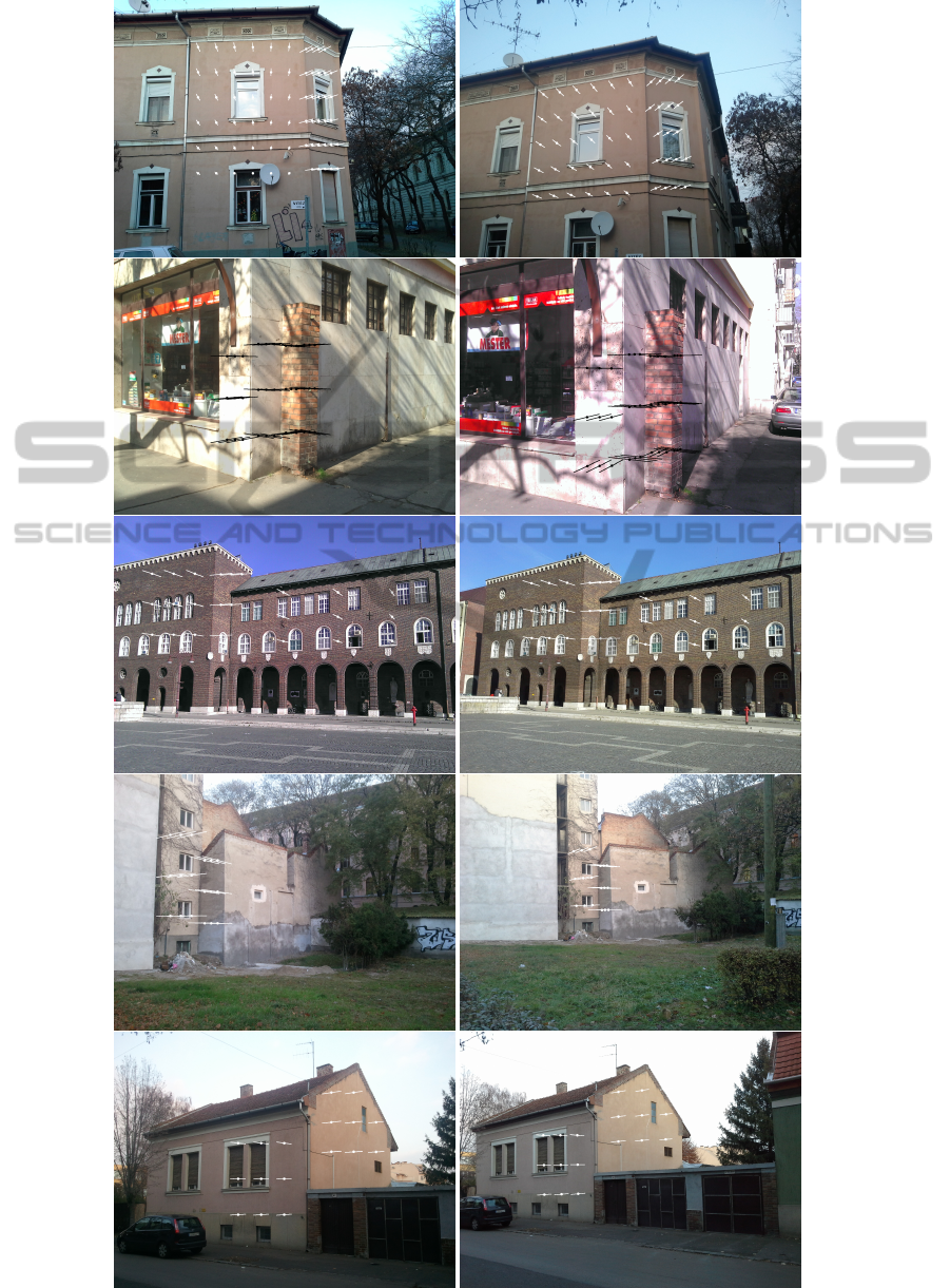
Figure 11: Estimated normals on planar surfaces.

OptimalSurfaceNormalfromAffineTransformation

313

can be achieved.

We reconstructed the plane normal via the afﬁne

transformation. The afﬁne parameters can eas-

ily be calculated from homography as it is shown

in (Moln

ar et al., 2014). The cameras are calibrated

via point-based 3D reconstruction by bundle adjust-

ment (B. Triggs and P. McLauchlan and R. I. Hart-

ley and A. Fitzgibbon, 2000). Then the normals are

computed by the proposed optimal method. We have

tested the OPT algorithm on ﬁve different stereo pairs

as it is visualized in Fig 11. They are short base-

line stereo images. The yielded normal vectors and

points of the planes are drawn on the input images.

The corresponding points on the wall surfaces are de-

noted by small dots, the normals are drawn both in-

side and outside the plane. The proposed method is

robust enough, it computes very accurately the sur-

face normals.

5 CONCLUSION AND FUTURE

WORK

Novel normal estimators have been proposed here that

can estimate the normal of a surface patch if two per-

spective images of the patch are given and the afﬁne

transformations of the projected patches are known

between the images. One of the proposed methods

is optimal: if only the elements of the afﬁne trans-

formation are contaminated with noise, the proposed

method (OPT) serves the optimal estimation in the

least square sense. It can be applied if the perspec-

tive cameras are fully calibrated.

It is also obvious that normal estimation is very

sensitive to the noise appearing in afﬁne transforma-

tions. In the future, we plan to improve the afﬁne

transformation estimation in order to get more real-

istic results. We will also deal with developing novel

reconstruction methods that use both point correspon-

dences and estimated normals in order to obtain a

more realistic 3D reconstruction of real-world 3D ob-

jects.

ACKNOWLEDGEMENT

This research was supported by the EU and the

State of Hungary, co-ﬁnanced by the European So-

cial Fund through project FuturICT.hu (grant no.: TA-

MOP4.2.2.C11/1/KONV20120013)

REFERENCES

B. Triggs and P. McLauchlan and R. I. Hartley and

A. Fitzgibbon (2000). Bundle Adjustment – A Mod-

ern Synthesis. In Triggs, W., Zisserman, A., and

Szeliski, R., editors, Vision Algorithms: Theory and

Practice, LNCS, pages 298–375. Springer Verlag.

orck,

A. (1996). Numerical Methods for Least Squares

Problems. Siam.

Faugeras, O. and Lustman, F. (1988). Motion and struc-

ture from motion in a piecewise planar environment.

Technical Report RR-0856, INRIA.

Fischler, M. and Bolles, R. (1981). RANdom SAmpling

Consensus: a paradigm for model ﬁtting with appli-

cation to image analysis and automated cartography.

Commun. Assoc. Comp. Mach., 24:358–367.

Fodor, B., Kaz

o, C., Zsolt, J., and Hajder, L. (2014). Normal

map recovery using bundle adjustment. IET Computer

Vision, 8:66 – 75.

Habbecke, M. and Kobbelt, L. (2006). Iterative multi-view

plane ﬁtting. In In VMV06, pages 73–80.

Habbecke, M. and Kobbelt, L. (2007). A surface-growing

approach to multi-view stereo reconstruction. In

CVPR.

Hartley, R. I. and Sturm, P. (1997). Triangulation. Computer

Vision and Image Understanding: CVIU, 68(2):146–

157.

Hartley, R. I. and Zisserman, A. (2003). Multiple View Ge-

ometry in Computer Vision. Cambridge University

Press.

Kreyszig, E. (1991). Differential geometry. Dover Publica-

tions.

Liu, H. (2012). Deeper Understanding on Solution Ambigu-

ity in Estimating 3D Motion Parameters by Homogra-

phy Decomposition and its Improvement. PhD thesis,

University of Fukui.

Malis, E. and Vargas, M. (2007). Deeper understanding of

the homography decomposition for vision-based con-

trol. Technical Report RR-6303, INRIA.

Moln

ar, J., Huang, R., and Kato, Z. (2014). 3d recon-

struction of planar surface patches: A direct solution.

ACCV Big Data in 3D Vision Workshop.

Tanacs, A., Majdik, A., Molnar, J., Rai, A., and Kato, Z.

(2014). Establishing correspondences between planar

image patches. In International Conference on Dig-

ital Image Computing: Techniques and Applications

(DICTA).

Woodham, R. J. (1978). Photometric stereo: A reﬂectance

map technique for determining surface orientation

from image intensity. In Image Understanding Sys-

tems and Industrial Applications, Proc. SPIE, volume

155, pages 136–143.

Yu, G. and Morel, J.-M. (2011). ASIFT: An Algorithm for

Fully Afﬁne Invariant Comparison. Image Processing

On Line, 2011.

Z. Megyesi, G. and D.Chetverikov (2006). Dense 3d re-

construction from images by normal aided matching.

Machine Graphics and Vision, 15:3–28.

VISAPP2015-InternationalConferenceonComputerVisionTheoryandApplications

314

APPENDIX

Algorithm for Optimal Normal Estimation. The

task is to minimize the cost function deﬁned in Eq. 10

with respect to normal vector n. The scale of the vec-

tor is arbitrary, only the direction of the normal is re-

quired. Such kind of problems are typically solved

using Lagrange-multipliers, however, it cannot be ap-

plied here since the derivatives become very difﬁcult.

For this reason, we utilize another constraint for the

normal: let the sum of the coordinates be 1. Thus, n

is written as n = [n

,1 − n

− n

]

. Eq. 10 can be

reformulated as,

argmin

∑

k=1



+ w

k,z

αm

+ αw

5,z

− a



where m = [n

], q

= [w

i,x

− w

i,z

i,y

− w

i,z

]

. (In-

dices x, y, and z denote the ﬁrst, second, and third

coordinates of vectors, respectively.)

The minima/maxima can be obtained by taking

the derivative with respect to vector m:

∑

k=1

= 0

where



+ w

k,z

αm

+ αw

5,z

− a





+ w

5,z

− (m

+ w

k,z

(αm

+ αw

5,z

)



After taking the lowest common multiple of the

fractions, the left side should be equal to zero as

∑

k=1

= 0, where



+ w

k,z

− a

αm

− a

αw

5,z





+ w

5,z

− (m

+ w

k,z



It can be simpliﬁed as

∑

k=1

= 0, where



− a

αq

) + (w

k,z

− a

αw

5,z

)





− (m

+ w

5,z

− w

k,z



This is an equation with a 2D-vector:

∑

k=1





k,x

− q

5,x



+ w

5,z

k,x

− w

k,z

5,x



k,y

− q

5,y



+ w

5,z

k,y

− w

k,z

5,y



= 0

where r =



− a

αq

) + (w

k,z

− a

αw

5,z

)



By introducing the m = [x, y]

notation, the vector

equation is modiﬁed as follows

∑

k=1

(Ω

x + Ψ

y + Γ

)



Ω

x + Ψ

y + Γ

Ω

x + Ψ

y + Γ



= 0

where

Ω

= q

k,x

− αq

5,x

= q

k,y

− αq

5,y

= w

k,z

− a

αw

5,z

Ω

= 0

= q

5,y

k,x

− q

k,y

5,x

= w

5,z

k,x

− w

k,z

5,x

Ω

= q

5,x

k,y

− q

k,x

5,y

= 0

= w

5,z

i,y

− w

i,z

5,y

The rows of the vector equation give two special

quadratic curves. They are written by their implicit

equations as

∑

k=1

∑

k=1

∑

k=1

xy +

∑

k=1

x +

∑

k=1

y +

∑

k=1

= 0, where A

Ω

, B

= Ψ

, C

= Ω

+Ψ

Ω

, D

= Ω

Ω

, E

= Ψ

+ Γ

and F

= Γ

, l ∈ 1,2.

They are special because A

= 0 and B

= 0.

The solution of the optimal method described in

the study (within appendix) is given by the intersec-

tion of two quadratic equations.

xy + D

x + E

y + F

= 0

xy + D

x + E

y + F

= 0

Parameter y can be obtained from the latter equation

y = −

+ D

x + F

x + E

Substituting y into the ﬁrst equation the following

expression is obtained



+ D

x + F

x + E



−

+ D

x + F

x + E

+ D

x −

+ D

x + F

x + E

+ F

= 0

If both sides are multiplied with (C

x + E

)

, then

the equation modiﬁes as follows

+ D

x + F

)

−



+ D

x + F



x + E

) +

x (C

x + E

)

− E



+ D

x + F



x + E

)

x + E

)

= 0

This is a fourth-order polynomial where the coef-

ﬁcients are as follows

: B

−C

−

+ D

− E

+ 2B

−

−C

+ 2D

−

− E

+ F

−C

− E

+ F

OptimalSurfaceNormalfromAffineTransformation

315

Remark that the equation C

x+E

= 0 can also be

considered. (In this case the ﬁrst equation is indepen-

dent from y.)

Figure 12: Quadratic curves.

An example for two quadratic curves with three

real intersections is visualized in Fig. 12. (The pa-

rameters of curves are B1 = −1.9055, C1 = 2.2632,

D1 = 2.8577, E1 = −9.4392, F1 = 7.7081, and A2 =

−2.2632, C2 = 1.9055, D2 = −4.2074, E2 = 2.3903,

F2 = −1.1190.)

VISAPP2015-InternationalConferenceonComputerVisionTheoryandApplications

316