Accelerated Ray Tracing using R-Trees

Dirk Feldmann

Department Scene Analysis, Fraunhofer IOSB, Ettlingen, Germany

Keywords:

Ray Tracing, R-Tree, Acceleration, Spatial Index, GPU, CUDA, Stackless Algorithm.

Abstract:

Efﬁcient ray tracing for rendering needs to minimize the number of redundant intersection tests between

rays and geometric primitives. Hence, ray tracers usually employ spatial indexes to organize the scene to be

rendered. The most popular ones for this purpose are currently kd-trees and bounding volume hierarchies,

for they have been found to yield best performances and can be adapted to contemporary GPU architectures.

These adaptations usually come along with costs for additional memory or preprocessing and comprise the

employment of stackless traversal algorithms.

R-trees are height-balanced spatial indexes with a ﬁxed maximum number of children per node and were

designed to reduce access to secondary memory. Although these properties make them compelling for GPU

ray tracing, they have not been used in this context so far.

In this article, we demonstrate how R-trees can accelerate ray tracing and their competitiveness for this task.

Our method is based on two traversal schemes that exploit the regularity of R-trees and forgo preprocessing or

alterations of the data structure, with the ﬁrst algorithm being moreover stackless. We evaluate our approach

in implementations for CPUs and GPUs and compare its performance to results we obtained by means of

kd-trees.

1 INTRODUCTION

Efﬁcient ray tracing needs to organize the objects of

a scene in such a way that there are as few as possi-

ble redundant intersection tests between rays and the

geometric primitives those objects consist of. This

is usually accomplished by employing spatial indexes

such as kd-trees, octrees, bounding volume hierar-

chies (BVHs) or various types of grids. Among these

data structures, kd-trees and BVHs have received

much attention in recent years, because they can be

implemented on contemporary GPUs in order to har-

ness their parallel computing capabilities.

R-trees (Guttman, 1984) were designed to index

spatial data in large databases and aim for reduc-

ing access to secondary memory. They are height-

balanced trees with arity usually > 2 and are used, for

instance, in modern database management systems,

like MySQL or Oracle Spatial (Oracle Corp., 2014a;

Oracle Corp., 2014b). Their regularity makes R-trees

well-suited for accelerating ray tracing, because it en-

ables efﬁcient stackless traversal schemes without ad-

ditional costs for extra pointers or extensive prepro-

cessing. Furthermore, the accompanying and poten-

tially high memory locality of the contained data ben-

eﬁts the architectures of today’s GPUs, whose perfor-

mances are sensitive to cache misses. But to the best

of our knowledge, R-trees have not yet been used as

acceleration data structures in ray tracing.

In this work we describe how R-trees can be em-

ployed to accelerate ray tracing of static scenes and

demonstrate their suitability for this task by means of

a CPU-based ray tracer and a CUDA-based one. We

present two different algorithms for ray traversal that

exploit the regularity of R-trees: The ﬁrst one is stack-

less, requires neither additional memory nor pointers

and is superior to a conventional stack-based traversal

scheme. Our second algorithm uses a small amount

of additional memory and improves the performance

of parallel ray tracing on GPUs in certain situations,

compared to our stackless method. We furthermore

compare the performance of our R-tree-based CPU

implementation with results we obtain by means of

kd-trees constructed using the popular surface area

heuristic. The results indicate that R-trees can be

competitive alternatives to kd-trees, but the traversal

of R-trees is additionally more convenient than those

of kd-trees or BVHs.

The remainder of this article is structured as fol-

lows: Section 2 summarizes the most important work

related to ours and gives a description of R-trees, for

these data structures appear to be less well known.

247

Feldmann D..

Accelerated Ray Tracing using R-Trees.

DOI: 10.5220/0005304802470257

In Proceedings of the 10th International Conference on Computer Graphics Theory and Applications (GRAPP-2015), pages 247-257

ISBN: 978-989-758-087-1

 2015 SCITEPRESS (Science and Technology Publications, Lda.)

(a) Bunny (b) Cathedral (c) Fairy (d) Conference

Figure 1: We employed the depicted test scenes and camera poses to evaluate the methods presented throughout this work: (a)

Standford Bunny, 69 632 triangles, (b) Sibenik Cathedral, 75 284 triangles, (c) a frame from the Utah Fairy Forest animation,

173 579 triangles, (d) Conference Room, 331 135 triangles.

In Section 3, we enter on aspects that need consider-

ation in order to use R-trees for accelerating ray trac-

ing. The two different algorithms for determining in-

tersections between rays and the geometric primitives

indexed by R-trees are presented in Section 4. In Sec-

tion 5, we evaluate the performance of our approach

and discuss the results. Additionally, we compare the

performance of our R-tree-based method for CPU ray

tracing to results we obtain when using kd-trees in-

stead. We conclude our work with a discussion and

prospects of future research in Section 6. The test

scenes we employed throughout this work are shown

in Figure 1.

2 BACKGROUND AND RELATED

WORK

By employing appropriate spatial indexes to keep the

number of redundant intersection tests of rays with

objects within a scene as small as possible, ray tracing

implementations on modern GPUs can achieve inter-

active frame rates and beyond for static scenes (Horn

et al., 2007). From the wide ﬁeld of spatial indexes,

which is covered in detail in (Samet, 2006), popu-

lar choices for organizing scenes have been various

kinds of grids, octrees, kd-trees, general BSP-trees

and bounding volume hierarchies (BVHs) (Suffern,

2007, p. 443). In the context of GPU ray tracing,

many researchers found kd-trees and BVHs to be the

most appropriate spatial indexes, because they yield

good performances (Wächter and Keller, 2006; Stich

et al., 2009) and can be adapted to processor architec-

tures of GPUs (Hachisuka, 2009; Hapala et al., 2011;

Hapala and Havran, 2011). The main difference be-

tween these two data structures is that BVHs partition

scenes with respect to the objects, whereas kd-trees

partition the underlying space.

R-trees (see Section 2.2) are spatial indexes that

share properties with BVHs as well as with kd-trees,

but have unique features of their own: Like BVHs,

R-trees organize objects based on their minimal axis-

aligned bounding boxes, but like in kd-trees, nodes

are split with respect to locations in space determined

by some heuristic (see Section 2.2.1). The resulting

splits, however, are not necessarily strictly binary par-

titions of the underlying space, but rather resemble

divisions in BVHs. In contrast to the latter ones, R-

trees are balanced in height and are designed analo-

gously to B-trees for reducing accesses to secondary

memory by increasing the locality of data in memory.

Furthermore, R-trees can be either constructed incre-

mentally by successive insertion of data or by using

methods for bulk loading all data at once (see (Sellis

et al., 1987; Arge et al., 2008), for instance).

Although the features of R-trees indicate a good

suitability for their application in ray tracing, which

has been pointed out in (Sylvan, 2010), these data

structures apparently have not been further examined

in this context so far. Surprisingly, they are not even

mentioned in recent surveys on ray tracing (Wald

et al., 2007; Hachisuka, 2009) or articles on splitting

BVHs (Stich et al., 2009).

2.1 KD-Trees and BVHs

Kd-trees have been reported to perform particularly

well in ray tracing when being constructed by means

of surface area heuristic (SAH) (MacDonald and

Booth, 1990), but their most severe disadvantage has

been for long time their high construction times. This

limitation has been alleviated by algorithms for more

efﬁcient construction (Wald and Havran, 2006). Al-

though the overall performance of kd-trees is fre-

quently superior to those of BVHs, because kd-trees

adapt better to the complexity of scenes, BVHs are

often preferred due to their simplicity (Wächter and

Keller, 2006; Stich et al., 2009). Other studies in-

dicate that BVHs perform better for tracing coherent

GRAPP2015-InternationalConferenceonComputerGraphicsTheoryandApplications

248

rays, whereas kd-trees are superior in case of incoher-

ent rays (Zlatuska and Havran, 2010).

When implementing kd-trees or BVHs on GPUs,

it is necessary to account for certain aspects of the

underlying processor architecture: The local memory

available to a GPU thread is signiﬁcantly less than to

programs running on CPUs. This impairs or even pre-

vents the allocation large amounts of local memory

and thus the employment of traversal algorithms that

rely on stacks or queues, for instance. Hence, vari-

ous methods for stackless kd-tree and BVH traversal

have been developed (Hapala et al., 2011; Hapala and

Havran, 2011), but they require additional processing

steps or extra storage for pointers or traversal states.

Furthermore, the performance of GPU kernels

strongly depends on the locality of data in memory

and the number of cache misses, because the latter

will delay the execution of a large number of threads

at once. Presenting data in a coherent way by means

of cache-friendly data structures and access patterns

is thus an important issue.

More details on the employment of kd-trees and

BVHs in ray tracing can be found in (Wächter and

Keller, 2006),(Hachisuka, 2009) and (Wald et al.,

2007), for example, where the latter article focuses

on ray tracing of dynamic scenes.

2.2 R-Trees

R-trees (Guttman, 1984) are height-balanced spatial

indexes related to B-trees (Bayer and McCreight,

1972). Data are stored based on their n-dimensional

minimal axis-aligned bounding boxes (AABBs),

which serve as keys and are commonly used to

support point-location and window queries (Samet,

2006). Like with B-trees, only the leaf nodes at the

lowest level l = 0 hold actual data. The entries of in-

termediate nodes at levels l > 0 point to nodes at the

next lower level l − 1. Except for the root located at

the topmost level L, each node contains at least m > 0

(usually m ≥ 2) and at most M > m entries. The root

may hold less than m entries, especially if the tree is

empty, but cannot contain more than M entries. Each

node maintains an n-dimensional AABB that encloses

the bounding boxes of the entries contained in that

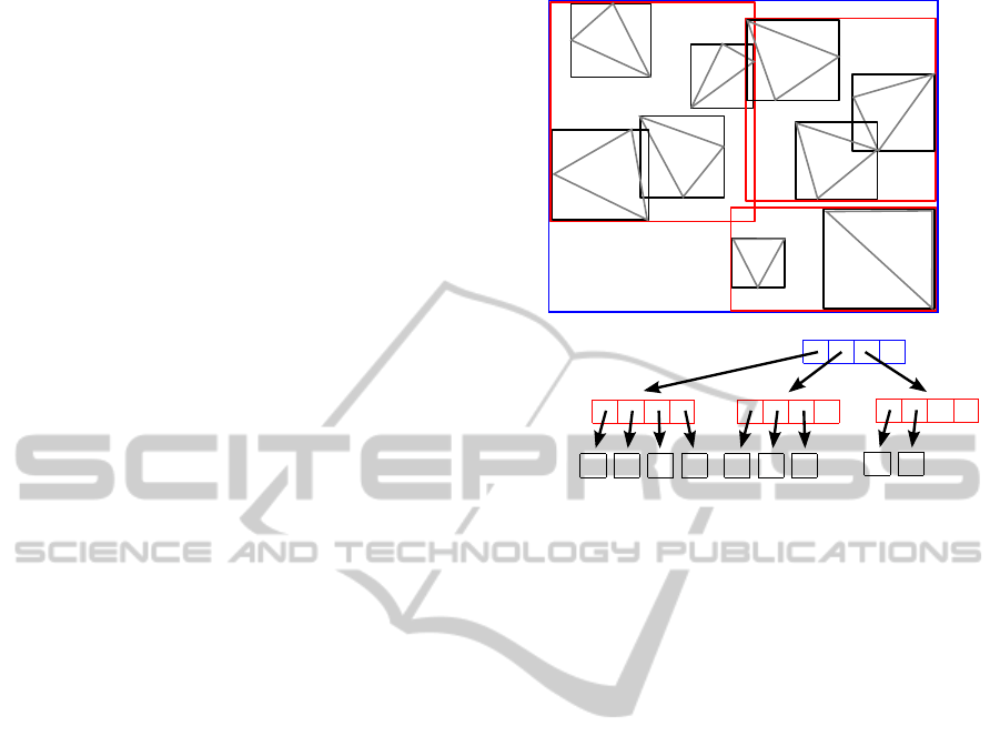
node. The structure of a 2D R-tree is illustrated in

Figure 2.

When data are inserted into an R-tree, leaf nodes

may overﬂow if they had to contain more than M en-

tries and hence must be split into two. The result-

ing extra leaf is inserted at the original leaf’s parent,

which in turn may overﬂow as well. This can trigger

cascades of node splits up to the root. If the root has

to be split, the tree grows by adding a new level L + 1

A C D G

B E F

l = 0

l = 1

l = 2

Figure 2: The data (triangles) A – I are stored in the leaf

nodes of a 2D R-tree with m = 2 and M = 4 at level l = 0

based on their AABBs. Entries of nodes at levels l > 0

point to nodes at the next lower level. Each node maintains

an AABB enclosing its entries (rectangles R

- R

and a new root, which receives the former root and its

new sibling become as the only children. Likewise,

if data are removed, nodes may underﬂow and must

hence be merged in order to satisfy the constraint of

holding at least m entries. Whenever an entry is added

or removed from a node, that node’s AABB must be

adjusted in such a way that it remains the minimal

AABB for all of the node’s entries. Except for the

increased complexity that comes along with splitting

nodes, the proceedings for adding data to or deleting

data from R-trees is the same as with B-trees.

In order to split nodes, there are various strategies

that directly inﬂuence the structure of an R-Tree and

thus its performance in subsequent ﬁnd operations.

These strategies usually try to minimize properties of

the AABBs of the resulting nodes, such as their vol-

ume, mutual overlap or surface, and are employed dif-

ferently or mixed in R-Tree variants.

2.2.1 R-Tree Construction

As illustrated in Figure 2, objects and their AABBs

stored in R-trees may overlap. Hence, the nodes,

which we identify with their maintained AABBs, may

also overlap each other at the same level. This im-

pedes ray traversal, because all paths in the tree start-

ing at locations where nodes overlap may lead to ge-

ometric primitives that may be intersected. In addi-

tion, nodes that include large amounts of dead space,

i.e., space only occupied by AABBs, but not by actual

AcceleratedRayTracingusingR-Trees

249

geometric primitives, must be tested for intersections

with rays, although the contained primitives may not

be intersected at all. Therefore, it is desirable to avoid

such situations by minimizing overlap and dead space

during the construction of R-trees. Since optimizing

for both these parameters at reasonable costs is in-

feasible in non-trivial situations, we have to rely on

heuristics to yield well-structured R-trees.

In the following, we brieﬂy present two existing

approaches on building R-trees by successive inser-

tion of data. At the level of leaf nodes, data are the

geometric primitives to be stored in the R-tree. At the

level of intermediate nodes, data are pointers to nodes

at the next lower level. In any case, data must always

be provided with their associated AABB.

For more details on the construction and split al-

gorithms, we refer to the original articles (Guttman,

1984; Beckmann et al., 1990).

The approach for constructing R-trees

in (Guttman, 1984) is formulated for AABBs in

2D and relies on selecting the node that requires the

least area enlargement when data are inserted. Ties

are resolved by selecting the node of least area. When

nodes need to be split due to overﬂow, the entries are

distributed in such a way that the total area occupied

by the two resulting nodes (and thus dead space) is

minimized.

The R

∗

-tree (Beckmann et al., 1990), a variant of

the R-tree, uses different strategies for choosing nodes

when inserting data at the levels of intermediate and

leaf nodes. In the former case, entries (i.e., other

nodes) are inserted at the node whose box needs least

area enlargement; ties are resolved by selecting the

node of least area. In case of leaf nodes, data are as-

signed to the node whose box will overlap least with

those of its siblings afterwards; ties are resolved by

using the node that requires least area enlargement.

Node splits in R

∗

-trees are performed by sorting

the entries of a node according to the minimum and

maximum values of their AABBs in each dimension

d. For each of the 2d sorts, a series of partitions into

two sets is constructed: The ﬁrst i entries in the sort,

where m ≤ i ≤ M +1 −m, are assigned to the ﬁrst set

of the i-th partition and the remaining M + 1 − i ones

to the second set. Each of these partitions along one

of the d axes represents a possible redistribution of

the entries from the overﬂowing node into two nodes.

The perimeters of all these candidates are summed up,

and the overﬂowing node is split along the axis where

the sum is minimal. Once the split axis has been de-

termined, the entries are distributed according to the

associated partition in which the two candidates have

least area overlap.

In addition, the R

∗

-tree extends the original R-

tree by using a technique called forced reinsert: As

a node ν overﬂows, instead of immediately splitting

it, its entries are sorted with respect to the distances

of their boxes’ centers from the center of ν’s box.

Depending on choice, the k entries with greatest or

least distance are removed (ejected) from ν. Starting

at the tree’s root, the ejected entries are then tried to

be reinserted at their respective levels. As a result,

they may become assigned to different parents at the

level of ν, because these new parents may have be-

come better choices with respect to the tree’s structure

and the criterion for selecting nodes. In this way, the

node occupancy is increased and potentially expen-

sive split operations are delayed. If the ejected entries

cannot be reinserted or if reinsertion would assign all

of them again to their original parent, a split must be

performed anyway.

In more recent work in (Beckmann and Seeger,

2009), the authors present the revised R

∗

-tree (RR

∗

tree). This variant employs modiﬁed strategies for

splitting and selecting nodes that supersede the need

for forced reinserts.

3 RAY TRACING USING

R-TREES

For the purpose of ray tracing, spatial indexes are

usually traversed to determine the object that is in-

tersected by the ray at least distance from the ori-

gin of that ray. R-trees have similarities to BVHs,

as they hold AABBs at every node, and ray traver-

sal is analog: Starting at the root, the maintained box

is checked for intersection with a given ray. If the

ray intersects the box, each of the n ∈ [m, M] chil-

dren’s boxes is tested for intersection with the ray, and

the process is recursively repeated for each positively

tested child node. In case the ray does not intersect

a box, the entries contained within that node do not

need to be considered any further, since they are not

intersected the ray either. The process terminates as

soon as all candidate objects at level l = 0 have been

tested.

Due to their structure, R-trees have certain proper-

ties that make them particularly interesting for accel-

erating ray tracing: In contrast to common BVHs or

kd-trees, R-trees are always balanced in height, i.e.,

all leaf nodes storing geometric primitives are located

at the same level (depth). Hence, paths from the root

towards leaves have constant lengths. Furthermore,

the number of nodes per level is limited by the value

chosen for M. This regularity allows to traverse R-

trees without maintaining an auxiliary stack and to

keep the memory consumption during traversal con-

GRAPP2015-InternationalConferenceonComputerGraphicsTheoryandApplications

250

stant, which is of special importance for parallel ray

tracing on GPUs, where the tree is traversed by mul-

tiple rays simultaneously.

3.1 Considerations for Ray Tracing

The equivalents of area and perimeter of 2D boxes

in 3D are volume and surface, respectively, and over-

lap is the common volume occupied by two or more

boxes. As pointed out in Section 2.2.1, the amounts of

dead space and overlap between nodes inﬂuences the

performance of R-trees. The amount of dead space

depends on the quality of approximations of the geo-

metric primitives by AABBs (and thus on the geom-

etry of the scene), on the choice of data assignment

to nodes and on the strategy for splitting nodes. The

latter two aspects also inﬂuence the amount of mutual

overlap.

Furthermore, R-tree nodes must be split if they ex-

ceed their limit of M entries, but the resulting nodes

must not contain less than m entries. Since m and M

determine how many entries must be checked if a ray

intersects the containing node, these two parameters

will inﬂuence the performance of R-trees as well.

Another aspect that inﬂuences ray tracing perfor-

mance is the order in which the n child nodes (entries)

are visited and is illustrated in Figure 3: Preferably,

the entries of R-tree nodes are stored in a coherent

block of memory, e.g., in an array, but visiting them

in their order in memory is not necessarily optimal.

Hence, the R-tree’s ray tracing performance changes

with the direction of rays. For the purpose of early

ray termination, the best sequence for visiting entries

would be the one obtained by sorting the contained

geometric primitives according to their distances from

a ray’s origin in increasing order. This order, however,

is usually not known in advance.

In summary, when using R-trees for ray tracing,

their performance is inﬂuenced by the following fac-

tors:

• the underlying geometry of the scene

• the strategy for assigning entries to nodes

• the strategy for splitting nodes

• the number of entries per node, i.e., m and M

• the order in which children of nodes are tested for

intersections with rays

4 RAY TRAVERSAL

Ray traversal in R-trees and its variants is similar to

the proceeding employed with BVHs (see Section 3).

ray

memory

A C

E F H IB

Figure 3: If the R-tree in Figure 2 is intersected by rays,

the order in which nodes are tested for intersection inﬂu-

ences the data structure’s performance. In case of vis-

iting nodes in the depicted memory order, the intersec-

tion at triangle I is closest to ray

, but is found only after

, A,C, D, G, R

, B, E, F, R

and H have been tested. The

intersection at A is closest to ray

and is found ﬁrst by

chance. Thus, testing the entries of R

and R

is needless.

ray

intersects C, but R

and its children need to be tested

for intersection as well, because these boxes are closer to

that ray’s origin.

In contrast to most trees and BVHs, R-trees are bal-

anced in height, which allows us to derive the follow-

ing relations:

The total number of nodes N in an R-tree of height

L + 1 holding at most M entries per node is given by

N =

∑

i=0

L+1

− 1

M − 1

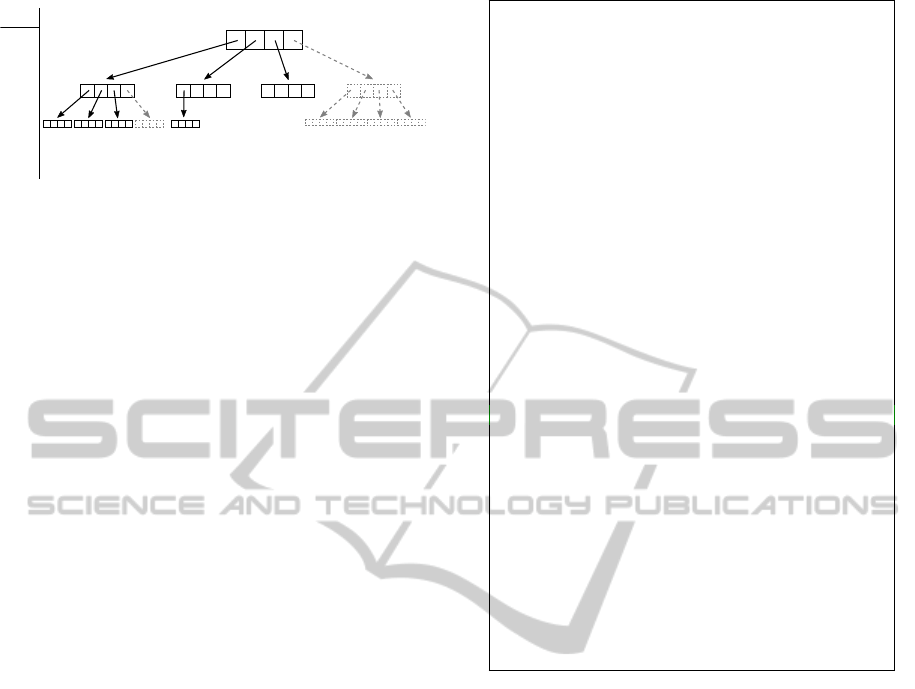
where N, L, M ∈ N. Starting at the root, we may num-

ber all nodes in level order from left to right, including

empty nodes (see Figure 4), and store the whole tree

sequentially in an array.

Since there are M

L−l

nodes at level l ≤ L, the ﬁrst

node at l is located at position ∆

(l) within the array,

where

∆

(l) =







0 l = L

L−(l+1)

∑

i=0

l < L

Given an intermediate node’s index n and level l > 0,

the index n

of its ﬁrst child/entry is

= n

(n) = (n − ∆

(l)) · M + ∆

(l − 1)

Likewise, if l < L, the index n

of a node’s parent is

= n

(n) =



(n − ∆

(l))



+ ∆

(l + 1)

AcceleratedRayTracingusingR-Trees

251

5 6

...

1 4

level

L-1

L-2

...

Figure 4: Level-order numbering of nodes in an R-tree with

M = 4. Empty nodes (dashed gray line style) must be num-

bered as well. Nodes from levels below L − 2 are omitted

for the sake of clarity.

The position k, 0 ≤ k < M, of n within its parent n

computed by

k = χ(n) = (n − ∆

(l)) mod M

Based on these relations, we devise the follow-

ing two algorithms for traversing R-trees and comput-

ing the closest intersection of the contained geometric

primitives with a given ray, if any such intersection

exists. The algorithm presented in Section 4.1 is a

straightforward implementation of depth-ﬁrst traver-

sal, but forgoes any additional stack. In Section 4.2,

we present a second traversal scheme that visits nodes

in the order of their distances from a ray’s origin.

Hereinafter, we assume that the primitives stored in

the R-trees are triangles, for they are very common in

rendering. A comparison of the performance of the

two algorithms is presented in Section 5.2.

4.1 Stackless Ray Traversal

Our algorithm for stackless depth-ﬁrst traversal of R-

trees is given in the pseudo code in Listing 1.

If the given ray intersects a box or a triangle, func-

tion intersects() returns the distance t from that

ray’s origin to the location of its ﬁrst intersection with

the object. Otherwise, the function returns ∞. The

result t

min

of the algorithm is the minimum of all dis-

tances obtained from intersections of a given ray with

triangles. If there are no intersections, t

min

= ∞.

The loop starting at line 21 locates the next sibling

of the current node n by examining whether n is the

last entry within its parent, i.e., χ(n) = M − 1. If so,

the process is repeated for the parent of n until either

an ancestor n

of n with χ(n

) < M −1 has been found

or the root node has been reached again. Otherwise,

if χ(n) < M − 1, n

is set to n. The algorithm then

continues with the next node n

+ 1. In this way, all

relevant nodes will be visited, and the algorithm is

guaranteed to terminate as soon as it has processed

the last entry of the root.

1 t

min

= ∞;

2 for (n = 0, l = L; n < N ; ) {

3 p roc e edW i thC h ild ? = false;

4 if ( ! isE mpt y Nod e (n) ) {

5 t = i nte rse cts ( ray , get Box (n)) ;

6 if ((t < ∞)∧ (t < t

min

)) {

7 if (l > 0) // vi sit ing int erm e dia te node

8 pro c eed W ith C hil d ? = true;

9 else { / / vis iti ng le af node

10 foreach ( tr ian gle o f n as tri ) {

11 t

tri

= i n ter sec ts ( ray , tri ) ;

12 if ((t

tri

< ∞) ∧ (t

tri

< t

min

))

13 t

min

= t

tri

;

14 } } } }

15 if ( pro c eed Wit h Chi l d ?) {

16 n = n

(n); // p roc ee d w it h fir st ch ild .. .

17 --l ; // ... at the next lo wer l eve l

18 } else {

19 n

= n;

20 // If n is las t entry wi thi n it s

pa re nt , .. .

21 while ((l < L)∧ (χ(n

) == M − 1)) {

(* @ \ l abe l { l bl : l ine - lo op }@*)

22 n

= n

(n); // ... try p are nt of n .. .

23 ++l; // ... at th e next hi ghe r lev el

24 }

25 if (l < L)

26 n = n

+ 1; // p roc eed w it h next sib lin g

27 else // or , if s till a t t he ro ot ,...

28 n = N; // . .. exit l oop at n ex t i ter ati on

29 }

30 }

31 return t

min

;

Listing 1: Pseudo code for our algorithm for stackless ray

traversal in R-trees. The syntax is borrowed from the pro-

gramming languages C/C++.

4.2 Ordered Ray Traversal

The algorithm in Listing 1 suffers from the problem

described in Section 3.1: Its performance depends on

the directions of rays and on the order in which child

entries are stored in memory. In case of primary rays,

for instance, the effect becomes apparent by differ-

ences in frame rates as the virtual camera is placed at

opposite locations of the scene, but looks at the same

point. However, if the mutual overlap between nodes

at the same level is low, there is a good chance that

an AABB located closer to a ray’s origin contains a

geometric primitive that is also intersected by that ray

at less distance than a primitive in an AABB further

away.

Based on this consideration, we devised another

algorithm for ray traversal in R-trees that relies on

sorting node entries and requires a small amount of

additional memory per ray: For each level l, we al-

locate a small stack and a pointer to its top and start

ray traversal at the root of the R-tree. Each entry of

GRAPP2015-InternationalConferenceonComputerGraphicsTheoryandApplications

252

a node at l > 0 that is intersected by a given ray is

pushed onto the stack of level l. We then sort the en-

tries on the stack according to the distances of their

ﬁrst intersection with that ray in decreasing order. The

entry with least distance is thus located at the top of

the stack, and the one with largest distance at the bot-

tom. We repeat the process with the ﬁrst node pointed

to by the stack pointer at level l. Note that this node

is located at l − 1. If we arrive at a leaf, we test the

contained triangles for intersection with the ray and

update the overall minimal distance t

min

, if necessary.

If a node turns out to be empty or is missed by the

ray, we proceed with the next node on the stack of

level l. When a stack runs empty, we ascend in the

tree by increasing the level and continue with nodes

from the corresponding stack. The algorithm termi-

nates as soon as the stack of the topmost level runs

empty.

Since each stack has to hold at most M entries at a

time, it can be implemented by an array of ﬁxed size.

Provided that the node entries and stack pointer are

numbers of the same data type, the amount of extra

memory required per ray is thus proportional to L ·

(M + 1) (at level l = 0, no stack is needed, though it

is convenient to provide one).

Pseudo code for this algorithm is presented in

Listing 2.

5 IMPLEMENTATION AND

EVALUATION

Our approach relies on R

∗

-trees (Beckmann et al.,

1990) in 3D, and we only use triangles as geometric

primitives for ray tracing static scenes. The numbers

for minimum and maximum entries per node are set to

m = 2 and M = 4, respectively, because this conﬁgu-

ration yielded best results in our experiments. The R-

trees are constructed on the CPU using pointers and

are packed according to the proceeding described in

Section 4 into a linear memory layout in a subsequent

step. Rays are not packeted (Wald et al., 2001), but

traced individually.

We implemented a simple CPU ray tracer de-

signed for execution on common desktop computers

using C++. The code relies in large parts on C++ tem-

plates, including some STL containers, and is mainly

optimized by the compiler alone. The ray tracer

merely allows basic parallel ray tracing by utilizing

the compiler’s OpenMP support in order to trace rays

from C different rows of the resulting image concur-

rently, where C is number of CPU cores.

Our CUDA ray tracer accesses R-trees via a set of

1D textures. Positions of the ﬁrst nodes ∆

(l) at each

1 t

min

= ∞;

2 sta cks [L + 1][M ] ; // e ntr ies at c urr ent l eve l

3 d ist anc es [L + 1]; // L + 1 is m or e c onv eni ent

4 sp [L + 1]; // s tac k p oi n te r s

5 for (n = 0, l = L; n < N ; ) {

6 if ( ! isE mpt y Nod e (n) ) {

7 if (l > 0) { // v i si t in g in t erm edi a te no de

8 sp [l ] = 0;

9 for (i = 0; i < M; ++i) {

10 n

= n

+ i;

11 if ( ! isE mpt y Nod e (n

)) {

12 t = i nte rse cts ( ray , get Box (n

));

13 if ((t < ∞)∧ (t < t

min

)) {

14 sta ck s [l ][ sp [l]] = n

;

15 dis tan ces [ sp [l]] = t ;

16 ++ sp[l ];

17 } }

18 }

19 sort ( s ta ck [l] , d is ta nces , sp [l ]) ;

20 } else { // v i si t in g l ea f node

21 foreach ( tr ian gle o f n as tri ) {

22 t

tri

= i n ter sec ts ( ray , tri ) ;

23 if ((t

tri

< ∞) ∧ (t

tri

< t

min

))

24 t

min

= t

tri

;

25 }

26 ++l; // d on e with th is le vel

27 } }

28 while ((l ≤ L)∧ (sp[l ] < 1) )

29 ++l ;

30 if ((l ≤ L)∧ (sp[l ] > 0) {

31 n = sta cks [l ][-- sp [l ]];

32 --l ; // n is now fro m th e ne xt lo wer l evel

33 } else

34 n = N ; // e xi t loop

35 }

36 return t

min

;

Listing 2: Pseudo code for our algorithm for ordered ray

traversal in R-trees. The algorithm requires additional

memory to maintain a small stack per level (arrays stacks

and sp). Function sort() performs in-place sorting of the

stack according to the distances of the intersections from

the ray’s origin.

each level l are precomputed and stored together with

the number of an R-tree’s maximum level L in the

constant memory area of the ray tracer’s kernel. In

all cases, we achieved best performance results when

running CUDA ray tracing kernels in a conﬁguration

of h blocks with 128 threads each, where h is the num-

ber of rows in the rendered image.

All measurements in the following were obtained

on a desktop computer with an Intel i7-4820K CPU at

3.7 GHz, 32 GB RAM and an NVIDIA GeForce GTX

780 graphics adapter with 3 GB memory (NVIDIA

Corp., 2014). Images were rendered at resolutions of

1024 × 1024 pixels, so that h = 1024 for all CUDA

kernel executions. The CPU ray tracer was executed

using all C = 8 processor cores available.

AcceleratedRayTracingusingR-Trees

253

5.1 Comparison of R-Tree Construction

Schemes

We constructed R

∗

-trees by successive insertion of tri-

angles and investigated the following strategies for se-

lecting nodes (cf. Section 2.2.1):

1. minVolume: minimize the volume enlargement

of nodes, regardless of their level. This is

the same strategy employed by the original R-

tree (Guttman, 1984).

2. minSurface: minimize the surface area enlarge-

ment of nodes. This corresponds to the sur-

face area heuristic (SAH) (MacDonald and Booth,

1990).

3. minOverlap: minimize the mutual overlap of

nodes, resolve ties by selecting the node that

needs least volume enlargement

4. R*-tree: minimize the volume enlargement at

intermediate nodes and the overlap at leaf nodes

5. R*-treeSrfc: similar to R*-tree, but minimize

the surface enlargement at intermediate nodes and

the overlap at leaf nodes

Alterations of the method for splitting nodes pre-

sented in (Beckmann et al., 1990), like using vol-

ume as measurements for determining split axes or re-

distributing entries, only impaired ray tracing perfor-

mance, and we thus relied on the original approach.

The inﬂuence of the node selection strategies on ray

tracing performance is summarized in Table 1. The

values were obtained by rendering our test scenes

from the ﬁxed camera poses shown in Figure 1 using

primary and shadow rays. For ray traversal by means

of our CPU implementation, we employed the stack-

less algorithm presented in Section 4.1, whereas our

GPU tracer relied on the method for ordered traversal

described in Section 4.2.

The results in Table 1 show that the two strate-

gies based on minimizing surfaces of AABBs, i.e.,

R*-treeSrfc and minSurface, are best for con-

structing R

∗

-trees for the purpose of ray trac-

ing. Minimizing the mutual overlap by means of

minOverlap diminished the performance consider-

ably, especially in case of the Bunny test scene

where CPU ray tracing performance was degraded by

≈ 2690% and our CUDA ray tracer even failed to

launch.

Furthermore, the results indicate a correlation be-

tween the insertion strategy and the geometry of a

scene and can be explained as follows:

Strategy minSurface favors the formation of boxes

of cubic shape, whereas minVolume prefers ﬂat boxes

that may have zero extension along one axis and thus

Table 1: The strategies for selecting nodes where trian-

gles are inserted into R-trees directly inﬂuence their struc-

ture and thus their performance in ray tracing. Values

were obtained by tracing primary and shadow rays. Using

minOverlap and the Bunny test scene, our CUDA kernels

failed to launch and we were unable to obtain results.

scene

minVolume

minSurface

minOverlap

R*-tree

R*-treeSrfc

CPU

Bunny 1.95 s 1.59 s 53.0 s 1.90 s 1.57 s

Cath. 6.40 s 4.95 s 13.6 s 5.39 s 3.54 s

Fairy 5.92 s 3.31 s 8.50 s 5.65 s 3.41 s

Conf. 3.99 s 3.30 s 5.79 s 3.94 s 3.01 s

GPU

Bunny 67 ms 63 ms – 71 ms 59 ms

Cath. 221 ms 162 ms 478 ms 201 ms 138 ms

Fairy 169 ms 98 ms 263 ms 158 ms 104 ms

Conf. 134 ms 113 ms 199 ms 134 ms 98 ms

zero volume, but which may have large surfaces. Both

strategies can reduce dead space, but minSurface

outperforms minVolume for the same reason that

makes SAH the preferred method for building kd-

trees: Provided the origins and directions of rays are

uniformly distributed in space, the conditional prob-

ability of a ray intersecting a box B

to intersect a

completely contained box B

is approximately pro-

portional to the ratio

S (B

)

S (B

)

of their surfaces S (B

), i ∈

{

1, 2

}

(see (MacDonald and Booth, 1990; Wald and

Havran, 2006)). Strategy minSurface chooses the

node where this probability is highest, and the inter-

section test between a ray and the outer box is thus

less likely to be redundant.

Strategy minOverlap assigns entries to nodes re-

gardless of dead space. This behavior is particularly

problematic at upper R-tree levels, where AABBs oc-

cupy potentially large volumes that may have to over-

lap due to the scene geometry. In case of the Bunny

scene, the virtual camera is moreover not located as

deep “inside” the R-tree as in the other scenes, but

is surrounded by only few AABBs from levels close

to L. Hence, much more tests for intersection with

rays and AABBs of large volume are needed, which

explains the poor performance of this method.

The strategies R*-tree and R*-treeSrfc are

composed of minOverlap and minVolume or

minSurface, respectively. However, only leaf nodes

are subject to minOverlap, and triangles are “di-

rected” already towards their respective parents based

on spatial locality and on (local) minimization of dead

space at higher levels. Optimizing for mutual over-

lap of leaf nodes results in a reduction of the num-

ber of paths that need to be followed during traver-

sal in R-trees. In this way, better performances are

yielded than in cases of minVolume and minSurface.

This proceeding has been reported to be a means

GRAPP2015-InternationalConferenceonComputerGraphicsTheoryandApplications

254

Table 2: Ray tracing performance of R-trees when omit-

ting forced reinserts during construction by means of

R*-treeSrfc strategy.

Bunny Cathedral Fairy Conference

CPU

1.92 s 4.42 s 3.81 s 3.01 s

(−23%) (−25%) (−12%) (±0%)

GPU 69 ms 154 ms 115 ms 105 ms

(−17%) (−12%) (−11%) (−7%)

of improving the performance of R

∗

-trees over R-

trees (Beckmann et al., 1990) and is conﬁrmed by our

results.

In addition, we found that forced reinserts used

with R

∗

-trees improve their structure and ray trac-

ing performance in most cases. The results we ob-

tained when sparing forced reinserts during construc-

tion of R-trees by means R*-treeSrfc strategy are

given in Table 2.

5.2 Comparison of Ray Traversal

Algorithms

We evaluated the two algorithms for tracing rays in R-

trees presented in Section 4 by means of our CPU and

GPU ray tracer, respectively. Performance was mea-

sured in the same way as described in Section 5.1 with

R-trees being constructed using the R*-treeSrfc

strategy and forced reinserts. In case of ordered ray

traversal, the auxiliary stacks were sorted using in-

sertion sort, because this sorting algorithm is easy

to implement, in-place and efﬁcient for small data

sets (Sedgewick, 2002). We also acquired timings by

using a conventional stack-based traversal algorithm

in our CPU implementation for comparison. The re-

sults are given in Table 3.

Table 3: Ray tracing performances of R-trees using the

traversal algorithms presented in Section 4 and a common

stack-based method (CPU ray tracer only).

scene stackless ordered stack

CPU

Bunny 1.57 s 1.82 s 2.09 s

Cathedral 3.54 s 4.23 s 5.94 s

Fairy 3.41 s 3.77 s 4.41 s

Conference 3.01 s 3.37 s 3.81 s

GPU

Bunny 65 ms 59 ms –

Cathedral 120 ms 138 ms –

Fairy 102 ms 104 ms –

Conference 98 ms 98 ms –

In most cases, best performance was achieved by

means of the stackless algorithm for ray traversal.

The ordered algorithm proved to be somewhat bet-

ter in case of the Bunny scene, in which the virtual

camera was placed at a location contained only by

few AABBs at higher levels of the R-tree. In the

remaining scenes, the camera was located deeper in-

side the R-trees. Hence, sorting nodes based on their

distances from the origins of the rays was needles

in most situations, and the accompanying overhead

diminished the ray tracing performance. However,

if we placed the virtual camera outside the AABBs

of R-trees, our ordered ray traversal outperformed

the stackless method. For instance, rendering the

Cathedral scene by means of our GPU ray tracer

from a virtual viewpoint outside the R-tree took 51

ms using the ordered traversal method, compared to

68 ms using the stackless algorithm. We therefore

propose to employ the presented traversal algorithms

for R-trees with respect to the position of the virtual

camera.

5.3 Comparison with KD-Trees

We compared the performance of R-trees in our CPU

ray tracer to timings we obtained from ray tracing by

means of kd-trees. The kd-trees were constructed us-

ing the local greedy surface area heuristic (SAH) and

the O



nlog

(n)



algorithm described in (Wald and

Havran, 2006). The method we employed to traverse

kd-trees is the stack-based algorithm given in (Hapala

and Havran, 2011). For the sake of better compara-

bility, we compare kd-tree traversal to a more simi-

lar stack-based algorithm for traversing R-trees. The

R-trees were again constructed using R*-treeSrfc

strategy and forced reinserts. Both traversal algo-

rithms are merely optimized to the effect that they

skip AABBs/half spaces which are further away from

a ray’s origin than any intersection with a triangle al-

ready encountered. The results are listed in Table 4

and were obtained by rendering our test scenes twice

from the ﬁxed camera poses shown in Figure 1: one

time by tracing primary rays only, and another time

using primary and shadow rays.

With the exception of the Bunny scene, the perfor-

Table 4: Timings in seconds from our comparison of R-trees

and kd-trees for ray tracing. Kd-trees were traversed using

a stack-based algorithm, and the results given for R-trees

apply to the stack-based traversal scheme also employed

in Section 5.2. The corresponding results for primary and

shadow rays are hence identical to those given in Table 3.

scene R

∗

-tree kd-tree

primary rays

Bunny 1.38 s 1.59 s

Cathedral 3.30 s 2.04 s

Fairy 2.59 s 2.23 s

Conference 2.43 s 2.14 s

primary and

shadow rays

Bunny 2.09 s 2.96 s

Cathedral 5.94 s 4.01 s

Fairy 4.41 s 3.96 s

Conference 3.81 s 3.46 s

AcceleratedRayTracingusingR-Trees

255

mance of kd-trees for ray tracing was superior to those

of R-trees. In case of Bunny, the better performance

of R-trees results from the small number of triangles

in that scene instead of from the position of the vir-

tual camera. In similar scenes consisting of less than

≈ 100000 triangles, but not presented in this work,

we found ray tracing by means of R-trees always to

be faster.

If we compared the results of stackless R-tree

traversal on CPUs in Table 3 to the corresponding

timings of stack-based kd-tree traversal in Table 4,

ray tracing using R-trees would be the faster method.

Since we did not consider alternatives for stackless

kd-tree traversal, we deem such a comparison be-

tween two fundamentally different algorithms and

any conclusions drawn from it inappropriate.

5.4 Construction Times

Although this work is not focused on the times

needed for constructing R

∗

-trees, it is worth mention-

ing that they are signiﬁcantly lower than the times

required for constructing SAH kd-trees by means of

the O



nlog

(n)



algorithm presented in (Wald and

Havran, 2006). We list the times from our implemen-

tation in Table 5 primarily to provide indications for

other researchers and potential future work.

Table 5: Timings in seconds required for constructing spa-

tial indexes containing our test scenes shown in Figure 1.

R-trees were constructed using forced reinserts.

scene R

∗

-tree kd-tree

Bunny 0.61 s 7.03 s

Cathedral 0.62 s 4.37 s

Fairy 1.63 s 20.02 s

Conference 2.91 s 27.59 s

In case of our test scenes Bunny and Conference,

the timings we obtained for kd-trees are remarkably

similar to those reported in (Wald and Havran, 2006)

(6.7 s and 30.5 s, respectively), although we have dif-

ferent hardware and an independent implementation.

The build times of the O (nlog(n)) algorithm the au-

thors presented in that work (3.2 s and 15.0 s, respec-

tively), are also much higher than the times required

for building R

∗

-trees. The latter in turn, are yet sig-

niﬁcantly higher than the times for building BVHs of

scenes corresponding to Bunny and Conference by

the sophisticated methods presented in (Wald, 2007).

6 CONCLUSIONS AND FUTURE

WORK

In this article, we gave a ﬁrst demonstration of the

suitability of R-trees for accelerating ray tracing. We

presented two algorithms for traversing R-trees that

exploit the regularity of these data structures in order

to compute intersections between the geometric prim-

itives stored within and rays. The method for stack-

less traversal requires neither to restructure the trees

nor extra memory for internal pointers or other. Al-

though our algorithm for ordered traversal may per-

form better with certain camera poses, the stackless

variant is particularly interesting due to its simplicity

and suitability for implementation on modern GPUs.

Ray traversal on GPUs might be further improved by

exploiting the ﬁxed path lengths of R-trees and care-

ful optimization. In addition, we have only traced in-

dividual rays and neglected the inﬂuence of ray coher-

ence so far, but packeting rays as presented in (Wald

et al., 2001; Günther et al., 2007) is likely to increase

ray tracing performance of R-trees.

Moreover, we investigated construction schemes

for R-trees and their inﬂuence on ray tracing perfor-

mance. We showed that altering the measure from

volume to surface in the original strategy of R

∗

-trees

for selecting nodes for data insertion results in a con-

siderable improvement. More sophisticated methods

for constructing R-trees, like the ones used with RR

∗

trees (Beckmann and Seeger, 2009), for example, or

bulk-loading data (Sellis et al., 1987; Arge et al.,

2008) might yield even better results. These methods

could probably beneﬁt from ideas designed for opti-

mizing BVHs, such as the ones presented in (Wächter

and Keller, 2006; Wald, 2007).

Our direct comparison with kd-trees showed that

these yield better performance results in most situ-

ations yet, but the employment of stackless meth-

ods for R-tree traversal appears preferable over stack-

based kd-tree traversal.

Major points for optimizing the performance of R-

trees in ray tracing might also be revealed by thor-

oughly investigations of the caching behavior of R-

trees on GPUs.

Considering the simplicity of ray traversal and the

potentially high data locality that result from their

regular structure, R-trees may become a competitive

choice for accelerating GPU ray tracing as more re-

search is done on this subject.

ACKNOWLEDGMENTS

We thank all persons who created the models we used

throughout this work and made them publicly avail-

able. Additionally, we give thanks to M. Pohl for her

helpful comments on this article.

GRAPP2015-InternationalConferenceonComputerGraphicsTheoryandApplications

256

REFERENCES

Arge, L., Berg, M. D., Haverkort, H., and Yi, K. (2008). The

Priority R-tree: A Practically Efﬁcient and Worst-case

Optimal R-tree. ACM Trans. Algorithms, 4(1):9:1–

9:30.

Bayer, R. and McCreight, E. (1972). Organization and

Maintenance of Large Ordered Indexes. Acta Infor-

matica, 1(3):173 – 189.

Beckmann, N., Kriegel, H.-P., Schneider, R., and Seeger, B.

(1990). The R*-tree: An Efﬁcient and Robust Access

Method for Points and Rectangles. In SIGMOD ’90:

Proceedings of the ACM SIGMOD International Con-

ference on Management of Data, volume 19(2), pages

322–331. ACM.

Beckmann, N. and Seeger, B. (2009). A Revised R*-tree in

Comparison with Related Index Structures. In Pro-

ceedings of the 2009 ACM SIGMOD International

Conference on Management of Data, SIGMOD ’09,

pages 799–812. ACM.

Günther, J., Popov, S., Seidel, H.-P., and Slusallek, P.

(2007). Realtime Ray Tracing on GPU with BVH-

based Packet Traversal.

Guttman, A. (1984). R-trees: A Dynamic Index Structure

for Spatial Searching. In SIGMOD ’84: Proceed-

ings of the ACM SIGMOD International Conference

on Management of Data, pages 47–57. ACM.

Hachisuka, T. (2009). Ray Tracing on Graphics Hard-

ware. Technical report, University of California at San

Diego.

Hapala, M., Davidovi

c, T., Wald, I., Havran, V., and

Slusallek, P. (2011). Efﬁcient Stack-less BVH Traver-

sal for Ray Tracing. In Proceedings of the 27th Spring

Conference on Computer Graphics, SCCG ’11, pages

7–12, New York, NY, USA. ACM.

Hapala, M. and Havran, V. (2011). Review: Kd-tree Traver-

sal Algorithms for Ray Tracing. Computer Graphics

Forum, 30(1):199–213.

Horn, D. R., Sugerman, J., Houston, M., and Hanrahan,

P. (2007). Interactive K-d Tree GPU Raytracing. In

Proceedings of the 2007 Symposium on Interactive 3D

Graphics and Games, I3D ’07, pages 167–174, New

York, NY, USA. ACM.

MacDonald, D. J. and Booth, K. S. (1990). Heuristics for

Ray Tracing Using Space Subdivision. The Visual

Computer, 6(3):153–166.

NVIDIA Corp. (2014). GeForce GTX 780 Speciﬁcations.

http://www.geforce.com/hardware/desktop-gpus/

geforce-gtx-780/speciﬁcations.

Oracle Corp. (2014a). MySQL 5.6 Reference

Manual. http://downloads.mysql.com/docs/

refman-5.6-en.a4.pdf.

Oracle Corp. (2014b). Oracle Spatial and Graph Devel-

oper’s Guide. http://docs.oracle.com/database/121/

SPATL/E49172-03.pdf.

Samet, H. (2006). Foundations of Multidimensional and

Metric Data Structures. Morgan Kaufmann, 1st edi-

tion.

Sedgewick, R. (2002). Algorithms in Java Parts I – IV.

Addison Wesley, 3rd edition.

Sellis, T. K., Roussopoulos, N., and Faloutsos, C.

(1987). The R+-Tree: A Dynamic Index for Multi-

Dimensional Objects. In Proceedings of the 13th In-

ternational Conference on Very Large Data Bases,

VLDB ’87, pages 507–518, San Francisco, CA, USA.

Morgan Kaufmann Publishers Inc.

Stich, M., Friedrich, H., and Dietrich, A. (2009). Spatial

Splits in Bounding Volume Hierarchies. In Proceed-

ings of the Conference on High Performance Graph-

ics 2009, HPG ’09, pages 7–13, New York, NY, USA.

ACM.

Suffern, K. (2007). Ray Tracing from the Ground Up. A. K.

Peters, Ltd., 1st edition.

Sylvan, S. (2010). R-trees: Adapting Out-Of-Core Tech-

niques to Modern Memory Architectures. Talk at

Game Developers Conference, http://gdcvault.com/

play/1012452/R-Trees-Adapting-out-of.

Wächter, C. and Keller, A. (2006). Instant Ray Tracing:

The Bounding Interval Hierarchy. In Proceedings

of the 17th Eurographics Conference on Rendering

Techniques, EGSR’06, pages 139–149, Aire-la-Ville,

Switzerland, Switzerland. Eurographics Association.

Wald, I. (2007). On Fast Construction of SAH-based

Bounding Volume Hierarchies. In Proceedings of the

2007 IEEE Symposium on Interactive Ray Tracing,

RT ’07, pages 33–40, Washington, DC, USA. IEEE

Computer Society.

Wald, I. and Havran, V. (2006). On Building Fast kd-Trees

for Ray Tracing, and on Doing That in O(N log N). In

Proceedings of the 2006 IEEE Symposium on Interac-

tive Ray Tracing, pages 61–70.

Wald, I., Mark, W. R., Günther, J., Boulos, S., Ize, T., Hunt,

W., Parker, S. G., and Shirley, P. (2007). State of the

Art in Ray Tracing Animated Scenes. In STAR Pro-

ceedings of Eurographics 2007, pages 89–116. The

Eurographics Association.

Wald, I., Slusallek, P., Benthin, C., and Wagner, M. (2001).

Interactive Rendering with Coherent Ray Tracing. In

Computer Graphics Forum, pages 153–164.

Zlatuska, M. and Havran, V. (2010). Ray Tracing on a

GPU with CUDA – Comparative Study of Three Al-

gorithms. In Proceedings of WSCG’2010, communi-

cation papers, pages 69–76.

AcceleratedRayTracingusingR-Trees

257