A Perceptual Measure of Illumination Estimation Error

Nikola Bani

c and Sven Lon

cari

Image Processing Group, Department of Electronic Systems and Information Processing, Faculty of Electrical Engineering

and Computing, University of Zagreb, 10000 Zagreb, Croatia

Keywords:

Color Constancy, Illumination Estimation, Image Enhancement, Perception, White Balancing.

Abstract:

The goal of color constancy is to keep colors invariant to illumination. An important group of color constancy

methods are the global illumination estimation methods. Numerous such methods have been proposed and

their accuracy is usually described by using statistical descriptors of illumination estimation angular error. In

order to demonstrate some of their fallacies and shortages, a very simple learning-based global illumination

estimation dummy method is designed for which the values of statistical descriptors of illumination estima-

tion error can be interpreted in contradictory ways. To resolve the paradox, a new performance measures is

proposed that focuses on perceptual difference between different illumination estimation errors. The effect of

ground-truth illumination distribution of the benchmark datasets on method evaluation is also demonstrated.

1 INTRODUCTION

Achieving color constancy means keeping image col-

ors invariant to scene illumination (Ebner, 2007) that

often alters them as shown in Fig. 1. This is impor-

tant before further image processing processing and it

is done in two steps: illumination estimation, which

is the crucial step, and chromatic adaptation i.e. re-

moving the illumination cast. In most cases for color

constancy the following image f formation process

with Lambertian assumption included is used:

(x) =

I(λ, x)R(x, λ)ρ

(λ)dλ (1)

where c is a color channel, x is a given image pixel,

λ is the wavelength of the light, ω is the visible spec-

trum, I(λ, x) is the spectral distribution of the light

source, R(x, λ) is the surface reﬂectance, and ρ

(λ) is

the camera sensitivity of the c-th color channel. Uni-

form illumination is often assumed and this leads to

removing x from I(λ, x). Then the observed color of

the light source e is:

e =









I(λ)ρ(λ)dλ. (2)

Only the direction of e is needed to perform

chromatic adaptation. Because the values of I(λ)

and ρ

(λ) are often unknown, calculating e is

an ill-posed problem. It is solved by making as-

sumptions, which has resulted in numerous color

(a) (b)

Figure 1: The same scene (a) with and (b) without illumi-

nation color cast.

constancy methods that can be split in at least two

groups. In the ﬁrst group are low-level statistics-

based methods like White-patch (WP) (Land, 1977)

and its improved version (Bani

c and Lon

cari

2014b), Gray-world (GW) (Buchsbaum, 1980),

Shades-of-Gray (SoG) (Finlayson and Trezzi,

2004), Grey-Edge (1st and 2nd order (GE1 and

GE2)) (Van De Weijer et al., 2007a), Weighted

Gray-Edge (Gijsenij et al., 2012), Color Spar-

row (CS) (Bani

c and Lon

cari

c, 2013), Color

Rabbit (CR) (Bani

c and Lon

cari

c, 2014a), using

color distribution (CD) (Cheng et al., 2014b). The

second group is composed of learning-based methods

like gamut mapping (pixel, edge, and intersection

based - PG, EG, and IG) (Finlayson et al., 2006),

using high-level visual information (HLVI) (Van

De Weijer et al., 2007b), natural image statis-

tics (NIS) (Gijsenij and Gevers, 2007), Bayesian

learning (BL) (Gehler et al., 2008), spatio-spectral

learning (maximum likelihood estimate (SL) and

136

Bani

c N. and Lon

cari

c S..

A Perceptual Measure of Illumination Estimation Error.

DOI: 10.5220/0005307501360143

In Proceedings of the 10th International Conference on Computer Vision Theory and Applications (VISAPP-2015), pages 136-143

ISBN: 978-989-758-089-5

 2015 SCITEPRESS (Science and Technology Publications, Lda.)

with gen. prior (GP)) (Chakrabarti et al., 2012),

exemplar-based learning (EB) (Joze and Drew,

2012), Color Cat (CC) (Bani

c and Lon

cari

c, 2015).

Most digital cameras have color constancy im-

plemented at the beginning of their image pipeline

so it operates on raw linear images (Gijsenij et al.,

2011). The implemented illumination estimation

method should be as precise and as fast as possible

because of the digital cameras’ limited computational

power. To determine which of the methods that are

fast enough should be used, accuracy comparison is

conducted by comparing statistical descriptors of il-

lumination estimation error. In this paper it is shown

that the mostly used descriptors may be misleading in

showing the methods’ practical performance.

For the sake of demonstration, a learning-based

global illumination estimation dummy method is de-

signed in a way to make two of the mostly used error

statistical descriptors give contradictory accounts on

the method’s accuracy. The contradiction is resolved

through discussion and by proposing a new illumina-

tion estimation performance measure. It combines the

good properties of some of the mostly used statisti-

cal descriptors and it takes the perceptual error into

account. Additionally, the negative effect of faulty

design of the benchmark datasets on comparison be-

tween different methods is also shown.

The paper is structured as follows: In Section II

the illumination estimation evaluation for global il-

lumination estimation methods is explained, in Sec-

tion III the dummy method intended to show the eval-

uation shortages is described and tested, in Section

IV the results are discussed, and in Section V a new

illumination estimation performance measure is pro-

posed.

2 ESTIMATION EVALUATION

2.1 Benchmark Datasets

The ﬁrst thing required to conduct a global illumina-

tion estimation method testing is a benchmark dataset.

Such dataset contains images and their ground-truth

illumination. The ground-truth illumination is usually

extracted by placing a calibration object into the scene

of each dataset image. The color of the achromatic

surface of the calibration object e.g. gray patches or

gray ball is then used as ground-truth illumination,

which is provided together with the images. Some of

the color constancy datasets are the GreyBall (Ciurea

and Funt, 2003), the ColorChecker (Gehler et al.,

2008) and its re-processed linear version (L. Shi,

2014), the NUS datasets (Cheng et al., 2014b). The

GreyBall dataset contains 11346 non-linear images,

which were taken from a video sequence. Very often

its linear version is used and it is obtained by perform-

ing an approximate inverse gamma correction of the

original images.

2.2 Error Description

Before a color constancy method is applied to an im-

age, ﬁrst the calibration object has to be masked out.

When the illumination estimation is performed, the

angle between it and the ground-truth illumination is

calculated and it serves as the angular error. After this

procedure is performed for all images of the dataset,

all of the per image angular errors are described by

means of statistical descriptors. Since the distribution

of the angular errors is not symmetrical, the most used

descriptor is the median of the angular error (Hordley

and Finlayson, 2004). Some other useful descriptors

include the mean and the trimean of the angular error.

In many cases a method having a lower median angu-

lar error is considered to be better than some other

method having a higher median angular error. Al-

though other illumination estimation error measures

exist e.g. different mathematical and perceptual dis-

tances, angular error is the most widely used error

measure and it has a high correlation with the sub-

jective measures (Gijsenij et al., 2009). However, ev-

ery objective error measure including angular error is

only an approximation of the perceived error because

the human vision color constancy is incomplete and

scene dependent.

3 THE DUMMY METHOD

3.1 Motivation

The reason for introducing a dummy method for

global illumination estimation is to show the fallacies

and shortages of the mostly used angular error statis-

tical descriptors. Since assumptions are needed for il-

lumination estimation methods, let’s consider several

facts and assumptions to show how foundations of the

dummy method might hypothetically be reasoned.

The ﬁrst one is that most common illuminations

are daylight, sunlight, or some kind of incandes-

cence. It has been shown that all of these have a

spectrum that can be modelled by the black-body ra-

diation (Judd et al., 1964) (Finlayson and Schaefer,

2001). Since assumptions are needed for the process

of illumination estimation, the next step is to assume

that some of the illuminations occur more often than

the other. This assumption can be conﬁrmed to some

APerceptualMeasureofIlluminationEstimationError

137

degree by looking at the distribution of real-life illu-

minations by taking the ground-truth illuminations of

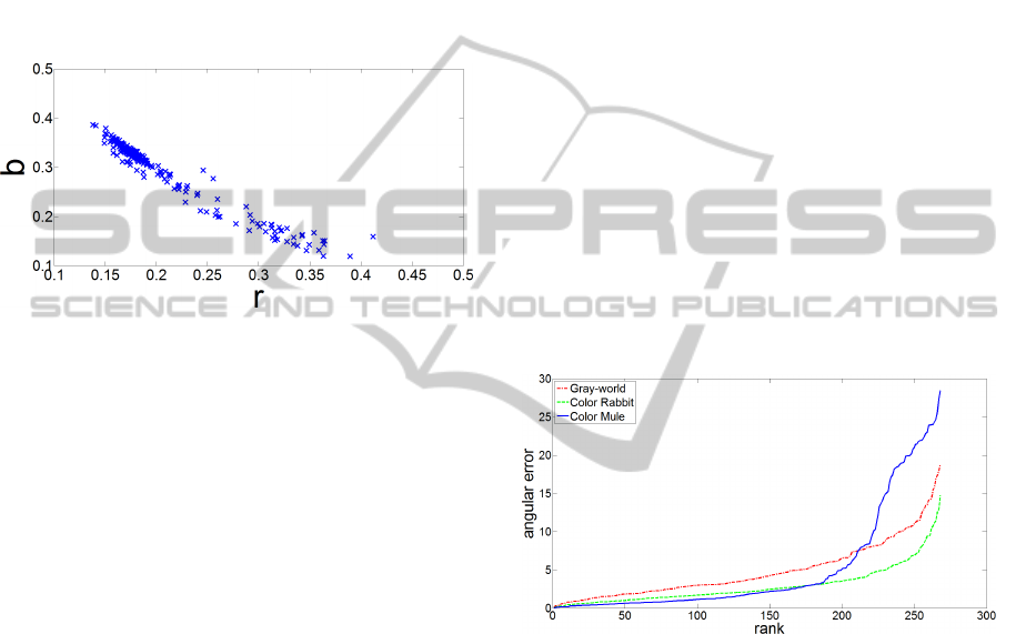
illumination estimation benchmark datasets. Fig. 2

shows the chromaticites of ground-truth illumination

of the Sony dataset (Cheng et al., 2014b). It can be

seen that some regions of the chromaticity space are

ﬁlled denser than the some other ones. This also holds

for the remaining NUS datasets (Cheng et al., 2014b)

and other datasets as well. Because it is evident that

some illuminations are more probable to occur, this

fact should be somehow used to obtain a better illu-

mination estimation.

Figure 2: The rb-chromaticities of the Sony dataset (Cheng

et al., 2014b) ground-truth illuminations.

3.2 Realization

Beside accuracy, computation speed is also consid-

ered in illumination estimation method design. In or-

der to assure that the dummy method is fast, it is de-

signed to assume that some illuminations occur more

often and therefore to simply select one ﬁxed illumi-

nation value, which is returned as illumination es-

timation for every given image. This value is ob-

tained in the learning process in which for each of

the ground-truth illuminations from the learning set

the angles between it and the rest of the learning set

ground-truth illuminations are calculated. The illumi-

nation that results in angles with the lowest median

angle is then selected to be the ﬁxed value. If the as-

sumption holds, then in the testing phase this value

should produce a relatively good illumination for the

majority of the images whose scenes are lit by the

most often illuminations.

Since this dummy method always stubbornly

gives the same illumination estimation, it is named

Color Mule (CM) for the purpose of a simpler nota-

tion in the rest of the paper.

3.3 Experimental Results

Illumination estimation is widely applied in digital

cameras at the beginning of the image processing

pipeline on raw images (Gijsenij et al., 2011) and

the image formation model used in Eq. (1) is lin-

ear. Therefore the NUS datasets with linear images

were used. Each of these datasets contains images

taken with a different camera. The well-known re-

processed linear version (L. Shi, 2014) of the original

ColorChecker dataset (Gehler et al., 2008) was not

used because in the majority of papers the black level

was erroneously not subtracted from the images be-

fore the testing procedure (Lynch et al., 2013), which

may lead to confusion when comparing the results of

methods from different publications.

Since the dummy CM method is a learning-based

one, it was tested by conducting a three-fold cross-

validation on the benchmark datasets. Table 1 shows

the angular error statistics for CM and other methods.

The results for other methods were taken from (Cheng

et al., 2014b) and (Cheng et al., 2014a). In terms of

median angular error, which is the most important,

CM outperforms all other methods on most of the

datasets. However, its trimean and especially mean

angular errors are far from being the best. Such dis-

agreement between the most important angular error

statistical descriptors opens the questions how to in-

terpret these results.

Figure 3: Comparison of sorted angular errors on the Sony

dataset (Cheng et al., 2014b) for the Gray-world, Color

Rabbit, and Color Mule.

4 DISCUSSION

4.1 Angular Error Distribution

When CM is excluded, then for 90% of all pairs com-

posed of methods from Table 1 it holds that if the

mean angular error of the pair’s ﬁrst method is greater

than the mean angular error of the second method,

then so is the median angular error and vice versa.

On the other hand, when considering only pairs where

one of the methods is CM, this holds for only 33% of

them indicating a discrepancy between the mean and

median.

The ﬁrst step to resolve the paradox of contradict-

VISAPP2015-InternationalConferenceonComputerVisionTheoryandApplications

138

Table 1: Angular error of selected low-level statistics-based methods, the proposed dummy method, and selected learning-

based methods on nine NUS benchmark image databases (lower is better).

Low-level statistics-based methods Learning-based methods

Method CR CD GW WP GGW GE1 GE2 CM PG EG IG ML GP NIS

Dataset Mean angular error (

◦

)

Canon1 3.09 2.93 5.16 7.99 3.16 3.45 3.47 5.43 6.13 6.07 6.37 3.58 3.21 4.18

Canon2 2.81 2.81 3.89 10.96 3.24 3.22 3.21 5.46 14.51 15.36 14.46 2.80 2.67 3.43

Fuji 2.94 3.15 4.16 10.20 3.42 3.13 3.12 5.79 8.59 7.76 6.80 3.12 2.99 4.05

Nikon1 3.06 2.90 4.38 11.64 3.26 3.37 3.47 6.26 10.14 13.00 9.67 3.22 3.15 4.10

Oly 2.65 2.76 3.44 9.78 3.08 3.02 2.84 5.29 6.52 13.20 6.21 2.92 2.86 3.22

Pan 2.89 2.96 3.82 13.41 3.12 2.99 2.99 5.70 6.00 5.78 5.28 2.93 2.85 3.70

Sam 2.94 2.91 3.90 11.97 3.22 3.09 3.18 5.72 7.74 8.06 6.80 3.11 2.94 3.66

Sony 2.88 2.93 4.59 9.91 3.20 3.35 3.36 5.07 5.27 4.40 5.32 3.24 3.06 3.45

Nikon2 3.57 3.81 4.60 12.75 4.04 3.94 3.95 7.66 11.27 12.17 11.27 3.80 3.59 4.36

Dataset Median angular error (

◦

)

Canon1 2.08 2.01 4.15 6.19 2.35 2.48 2.44 1.88 4.30 4.68 4.72 2.80 2.67 3.04

Canon2 1.86 1.89 2.88 12.44 2.28 2.07 2.29 1.87 14.83 15.92 14.72 2.32 2.03 2.46

Fuji 1.84 2.15 3.30 10.59 2.60 1.99 2.00 2.15 8.87 8.02 5.90 2.70 2.45 2.95

Nikon1 1.91 2.08 3.39 11.67 2.31 2.22 2.19 1.89 10.32 12.24 9.24 2.43 2.26 2.40

Oly 1.79 1.87 2.58 9.50 2.15 2.11 2.18 1.71 4.39 8.55 4.11 2.24 2.21 2.17

Pan 1.70 2.02 3.06 18.00 2.23 2.16 2.04 1.59 4.74 4.85 4.23 2.28 2.22 2.28

Sam 1.88 2.03 3.00 12.99 2.57 2.23 2.32 1.99 7.91 6.12 6.37 2.51 2.29 2.77

Sony 2.10 2.33 3.46 7.44 2.56 2.58 2.70 1.81 4.26 3.30 3.81 2.70 2.58 2.88

Nikon2 2.42 2.72 3.44 15.32 2.92 2.99 2.95 2.38 10.99 11.64 11.32 2.99 2.89 3.51

Dataset Trimean angular error (

◦

)

Canon1 2.56 2.22 4.46 6.98 2.50 2.74 2.70 2.47 4.81 4.87 5.13 2.97 2.79 3.30

Canon2 2.17 2.12 3.07 11.40 2.41 2.36 2.37 2.71 14.78 15.73 14.80 2.37 2.18 2.72

Fuji 2.13 2.41 3.40 10.25 2.72 2.26 2.27 2.97 8.64 7.70 6.19 2.69 2.55 3.06

Nikon1 2.23 2.19 3.59 11.53 2.49 2.52 2.58 2.87 10.25 11.75 9.35 2.59 2.49 2.77

Oly 2.01 2.05 2.73 9.54 2.35 2.26 2.20 2.60 4.79 10.88 4.63 2.34 2.28 2.42

Pan 2.12 2.31 3.15 14.98 2.45 2.25 2.26 2.64 4.98 5.09 4.49 2.44 2.37 2.67

Sam 2.18 2.22 3.15 12.45 2.66 2.32 2.41 2.79 7.70 6.56 6.40 2.63 2.44 2.94

Sony 2.26 2.42 3.81 8.78 2.68 2.76 2.80 2.40 4.45 3.45 4.13 2.82 2.74 2.95

Nikon2 2.67 3.10 3.69 13.80 3.22 3.21 3.38 4.96 11.11 12.01 11.30 3.11 2.96 3.84

ing statistical descriptor values is to look at the actual

angular errors. Fig. 3 shows the sorted angular er-

rors on the Sony (Cheng et al., 2014b) dataset for the

well-known Gray-World method, the accurate Color

Rabbit method, and the dummy Color Mule method.

It can be seen that for about slightly more than half

of the images CM results in a relatively low angular

error, which in turn results in a low median. How-

ever, the tail of CM’s angular error distribution con-

tains signiﬁcantly higher values than the tails of other

methods’ angular error distributions. Since the me-

dian does not consider this, it is automatically ren-

dered not to be informative enough to provide a good

description of CM’s performance.

4.2 Perceptual Signiﬁcance of the

Angular Error

It might seem that for CM a better descriptor would

be the mean angular error. But before drawing con-

clusions like this one, ﬁrst the perceptual signiﬁcance

of the angular error should be considered. Under We-

ber’s law (Weber, 1846) the just noticeable difference

increases linearly with the absolute error as was con-

ﬁrmed in (Gijsenij et al., 2009). In the same paper

a simple example is given to clarify this: while the

difference between the results of algorithms with er-

rors of 3

◦

and 4

◦

is noticeable to most people, this is

hardly the case if these errors are 15

◦

and 16

◦

. This

is explained even further by obtained experimental re-

sults. If ε

min

and ε

max

are two illumination estimation

angular errors with ε

max

being the greater one, then

the difference ∆ε = ε

max

− ε

min

between them is no-

ticeable if it is at least 0.06 · ε

max

. This means that for

an noticeable improvement an error ε has to be low-

ered to

= (1 − 0.06) · ε = 0.94 · ε. (3)

For a noticeable decline the error ε has to be raised to

∗

1 − 0.06

· ε =

0.94

· ε. (4)

This shows the weakness of the mean angular er-

ror, which does not take into account the percep-

APerceptualMeasureofIlluminationEstimationError

139

tual difference as can be demonstrated by choosing a

method and creating its degraded version. The degra-

dation process is done by increasing the all of the ini-

tial method’s angular errors by 5%, which is less then

needed for a noticeable difference. By degrading the

Color Rabbit method on the Sony dataset, its mean

angular error raises from 2.88

◦

to 3.02

◦

even though

there is no noticeable difference between the results

of the initial and degraded method on individual im-

ages. If the degradation is performed in another way

by choosing ﬁve errors that are less than 1

◦

and in-

creasing them by 5

◦

, the Color Rabbit’s mean raises

to 3.01

◦

, which is less than 3.02

◦

in the ﬁrst case, but

it nevertheless results in ﬁve noticeable and serious il-

lumination estimation accuracy deteriorations in con-

trast to the ﬁrst degradation way.

Since both the mean and the median angular errors

have shortages with respect to describing a method’s

performance, a better measure containing the best of

these two statistical descriptors and taking into ac-

count the perceptual difference should be devised.

5 PROPOSED MEASURE

5.1 Deﬁnition

To resolve the paradox caused by describing the Color

Mule’s performance using the mean and median an-

gular errors, we propose a new error measure based

on the angular errors and two facts about their percep-

tion. The ﬁrst one is that an angular error below 1

◦

not noticeable (Finlayson et al., 2005) (Fredembach

and Finlayson, 2008). The errors ε ∈ [0

◦

, 1

◦

] should

therefore not be penalized. The second fact is the al-

ready mentioned linear increase of the just noticeable

difference with the absolute error as stated by Weber’s

law and described by Eq. (3) and Eq. (4). Based on

these equations an error ε > 1 can be described by us-

ing the number of just noticeable differences n that

have led to its distancing from the 1

◦

ε =



0.94



. (5)

Since n takes into account the actual linear percep-

tual difference caused by the angular error, we pro-

pose it to be the basis for describing the perceptual

error of the illumination estimation. It is calculated as

follows:

n = log

0.94

ε =

lnε

0.94

. (6)

Since

0.94

is a constant, it has no impact on errors

comparison. Therefore a slightly modiﬁed difference

description m can be used:

m = nln

0.94

= lnε. (7)

The expression in Eq. (7) can be additionally inter-

preted by looking at its derivative:

dm =

dε

. (8)

As expected from the previous discussion, the in-

crease of the perceptual difference is directly pro-

portional to the increase of the angular error and in-

versely proportional to the angular error that is in-

creased. Like in Weber’s law, this means that in order

to achieve the same perceptual difference, for higher

angular errors the angular increase has to be larger

then for the lower angular errors.

For the general case where ε > 0 the measure m

from Eq. (7) is given as follows:

m =

(

0 if 0 ≤ ε ≤ 1

lnε if ε > 1

. (9)

The simplest way to use this measure to describe a

methods performance on an image dataset is to calcu-

late its mean value for all angular errors. The advan-

tage of this mean over the mean angular error is that

it considers the perceptual differences between differ-

ent angular errors and its advantage over the median

angular error is that is considers all angular errors.

5.2 Experimental Results

Table 2 shows the value of the proposed measure

for the dummy Color Mule and some of the selected

methods. The ranking between other methods ex-

cluding Color Mule remained the same as the rank-

ing based on the median angular error. Color Mule

is now ranked lower than the Color Rabbit and Color

Distribution methods, but higher than the Gray-world

and White-patch methods. The exception is only the

Olympus dataset where the Gray-world method out-

performs Color Mule. It can be seen that the proposed

measure penalizes the angular error distribution tail

of the proposed method, but not as strict as the mean

angular error. On the other hand it does not simply

disregard it as the median angular error thus avoiding

confusion. The sorted proposed measure values on

the Sony dataset for several chosen methods can be

seen in Fig. 4.

5.3 Dataset Illumination Distribution

The proposed measure mostly resolves the paradox

that resulted from the proposed method. However,

VISAPP2015-InternationalConferenceonComputerVisionTheoryandApplications

140

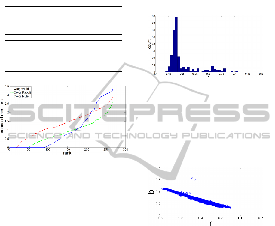
Table 2: Proposed measure for several selected methods on

nine NUS benchmark image databases (lower is better).

Selected methods

Method CR CD GW WP CM

Dataset Proposed measure

Canon1 0.8875 0.8233 1.2945 1.7062 1.0165

Canon2 0.7823 0.8003 1.0950 2.0899 1.0361

Fuji 0.8058 0.8419 1.1384 2.0114 1.0748

Nikon1 0.8418 0.8785 1.1658 2.0879 1.1010

Oly 0.7442 0.7667 0.9843 1.9116 0.9980

Pan 0.7878 0.8409 1.0887 2.3174 0.9959

Sam 0.8223 0.8256 1.1042 2.2348 1.0723

Sony 0.8345 0.8485 1.3177 1.8817 0.9565

Nikon2 1.0194 1.0708 1.2258 2.3318 1.2780

Figure 4: Comparison of sorted proposed measure values on

the Sony dataset (Cheng et al., 2014b) for the Gray-world,

Color Rabbit, and the proposed method.

there is still the question how such a simple method

could have outperformed much more sophisticated

methods in terms of median angular error and even

some of the methods in terms of the proposed mea-

sure. The reason for this may be found in the

dataset ground-truth illumination as can be demon-

strated with the Sony dataset. In Fig. 2 it can be

seen that for the Sony dataset most of the of ground-

truth illumination chromaticities lay in the left part of

the chromaticity space region. This can be demon-

strated even further quantitatively by looking at the

histogram of the red chromaticity component values

of the ground-truth illumination in Fig. 5. Now the

density of certain regions becomes even more clear:

e.g. over 86% of the values are less than 0.27. Such

density in a relatively small region can hardly be

found in other benchmark datasets.

The proposed method simply (ab)uses this de-

sign fault that happened in image selection during

the dataset creation and by choosing a good illumina-

tion value, it successfully covers most of the ground-

truth illuminations in the testing process. This is

also the reason why the median angular error could

have been so low when compared to the one of other

methods. At the same time the number of images

whose ground-truth illuminations were distanced fur-

ther from the majority of other ground-truth illumi-

nations was small, but the errors was big enough to

cause a very high mean angular error regardless of

the low median.

Figure 5: Histogram of the red chromaticity component val-

ues for the Sony (Cheng et al., 2014b)dataset ground-truth

illumination chromaticities.

When using non-linear images of the GreyBall

dataset (Ciurea and Funt, 2003), which has evenly

spread ground-truth illuminations as shown in Fig. 6,

the dummy Color Mule method performs very poor

in terms of all performance measures including the

proposed one as shown in Table 3. For the GreyBall

dataset the proposed measure is consistent with the

existing ones.

Figure 6: The rb-chromaticities of the GreyBall

dataset (Ciurea and Funt, 2003) ground-truth illumi-

nations.

6 CONCLUSIONS AND FUTURE

RESEARCH

A new illumination estimation accuracy measure has

been proposed. In contrast to the most widely

used angular error statistical descriptors, the proposed

measure takes into account the perceptual difference

between various errors. The good properties of mean

and median are used by using all angular errors and

penalizing them based on perceptual difference. Ad-

ditionally, a method has been proposed that shows the

importance of the representativity of the real-world

scene illuminations in the benchmark datasets.

APerceptualMeasureofIlluminationEstimationError

141

Table 3: Different performance measures for different color

constancy methods on the original GreyBall dataset (Ciurea

and Funt, 2003) (lower is better).

method mean (

◦

) median (

◦

) proposed

do nothing 8.28 6.70 1.6209

Low-level statistics-based methods

GW 7.87 6.97 1.8017

WP 6.80 5.30 1.5385

SoG 6.14 5.33 1.5732

general GW 6.14 5.33 1.5732

GE1 5.88 4.65 1.5013

GE2 6.10 4.85 1.5343

Learning based methods

PG 7.07 5.81 1.6478

EG 6.81 5.81 1.6616

IG 6.93 5.80 1.6510

NIS 5.19 3.93 1.3369

EB 4.38 3.43 1.1924

CM 9.78 8.65 1.9069

ACKNOWLEDGEMENTS

This research has been partially supported by the Eu-

ropean Union from the European Regional Develop-

ment Fund by the project IPA2007/HR/16IPO/001-

040514 ”VISTA - Computer Vision Innovations for

Safe Trafﬁc.”

REFERENCES

Bani

c, N. and Lon

cari

c, S. (2013). Using the Random

Sprays Retinex Algorithm for Global Illumination Es-

timation. In Proceedings of The Second Croatian

Computer Vision Workshop (CCVW 2013), pages 3–7.

University of Zagreb Faculty of Electrical Engineer-

ing and Computing.

Bani

c, N. and Lon

cari

c, S. (2014a). Color Rabbit: Guid-

ing the Distance of Local Maximums in Illumina-

tion Estimation. In Digital Signal Processing (DSP),

2014 19th International Conference on, pages 345–

350. IEEE.

Bani

c, N. and Lon

cari

c, S. (2014b). Improving the White

patch method by subsampling. In Image Processing

(ICIP), 2014 21st IEEE International Conference on,

pages 605–609. IEEE.

Bani

c, N. and Lon

cari

c, S. (2015). Color Cat: Remember-

ing Colors for Illumination Estimation. Signal Pro-

cessing Letters, IEEE, 22(6):651–655.

Buchsbaum, G. (1980). A spatial processor model for object

colour perception. Journal of The Franklin Institute,

310(1):1–26.

Chakrabarti, A., Hirakawa, K., and Zickler, T. (2012). Color

constancy with spatio-spectral statistics. Pattern Anal-

ysis and Machine Intelligence, IEEE Transactions on,

34(8):1509–1519.

Cheng, D., Prasad, D., and Brown, M. S. (2014a). On Illu-

minant Detection.

Cheng, D., Prasad, D. K., and Brown, M. S. (2014b). Il-

luminant estimation for color constancy: why spatial-

domain methods work and the role of the color distri-

bution. Journal of the Optical Society of America A,

31(5):1049–1058.

Ciurea, F. and Funt, B. (2003). A large image database

for color constancy research. In Color and Imaging

Conference, volume 2003, pages 160–164. Society for

Imaging Science and Technology.

Ebner, M. (2007). Color Constancy. The Wiley-IS&T Se-

ries in Imaging Science and Technology. Wiley.

Finlayson, G. D., Hordley, S. D., and Morovic, P. (2005).

Colour constancy using the chromagenic constraint.

In Computer Vision and Pattern Recognition, 2005.

CVPR 2005. IEEE Computer Society Conference on,

volume 1, pages 1079–1086. IEEE.

Finlayson, G. D., Hordley, S. D., and Tastl, I. (2006). Gamut

constrained illuminant estimation. International Jour-

nal of Computer Vision, 67(1):93–109.

Finlayson, G. D. and Schaefer, G. (2001). Solving for

colour constancy using a constrained dichromatic re-

ﬂection model. International Journal of Computer Vi-

sion, 42(3):127–144.

Finlayson, G. D. and Trezzi, E. (2004). Shades of gray and

colour constancy. In Color and Imaging Conference,

volume 2004, pages 37–41. Society for Imaging Sci-

ence and Technology.

Fredembach, C. and Finlayson, G. (2008). Bright chroma-

genic algorithm for illuminant estimation. Journal of

Imaging Science and Technology, 52(4):40906–1.

Gehler, P. V., Rother, C., Blake, A., Minka, T., and Sharp, T.

(2008). Bayesian color constancy revisited. In Com-

puter Vision and Pattern Recognition, 2008. CVPR

2008. IEEE Conference on, pages 1–8. IEEE.

Gijsenij, A. and Gevers, T. (2007). Color Constancy us-

ing Natural Image Statistics. In Computer Vision and

Pattern Recognition, 2008. CVPR 2008. IEEE Confer-

ence on, pages 1–8.

Gijsenij, A., Gevers, T., and Lucassen, M. P. (2009). Per-

ceptual analysis of distance measures for color con-

stancy algorithms. JOSA A, 26(10):2243–2256.

Gijsenij, A., Gevers, T., and Van De Weijer, J. (2011).

Computational color constancy: Survey and exper-

iments. Image Processing, IEEE Transactions on,

20(9):2475–2489.

Gijsenij, A., Gevers, T., and Van De Weijer, J. (2012). Im-

proving color constancy by photometric edge weight-

ing. Pattern Analysis and Machine Intelligence, IEEE

Transactions on, 34(5):918–929.

Hordley, S. D. and Finlayson, G. D. (2004). Re-evaluating

colour constancy algorithms. In Pattern Recognition,

2004. ICPR 2004. Proceedings of the 17th Interna-

tional Conference on, volume 1, pages 76–79. IEEE.

Joze, H. R. V. and Drew, M. S. (2012). Exemplar-Based

Colour Constancy. In British Machine Vision Confer-

ence, pages 1–12.

Judd, D. B., MacAdam, D. L., Wyszecki, G., Budde, H.,

Condit, H., Henderson, S., and Simonds, J. (1964).

Spectral distribution of typical daylight as a function

VISAPP2015-InternationalConferenceonComputerVisionTheoryandApplications

142

of correlated color temperature. JOSA, 54(8):1031–

1040.

L. Shi, B. F. (2014). Re-processed Version of the Gehler

Color Constancy Dataset of 568 Images.

Land, E. H. (1977). The retinex theory of color vision. Sci-

entiﬁc America.

Lynch, S. E., Drew, M. S., and Finlayson, k. G. D. (2013).

Colour Constancy from Both Sides of the Shadow

Edge. In Color and Photometry in Computer Vision

Workshop at the International Conference on Com-

puter Vision. IEEE.

Van De Weijer, J., Gevers, T., and Gijsenij, A. (2007a).

Edge-based color constancy. Image Processing, IEEE

Transactions on, 16(9):2207–2214.

Van De Weijer, J., Schmid, C., and Verbeek, J. (2007b). Us-

ing high-level visual information for color constancy.

In Computer Vision, 2007. ICCV 2007. IEEE 11th In-

ternational Conference on, pages 1–8. IEEE.

Weber, E. (1846). Der Tastsinn und das Gemeingef

uhl.

Handw

orterbuch der Physiologie, 3(2):481–588.

APerceptualMeasureofIlluminationEstimationError

143