Fast Rotation Invariant Object Detection with Gradient based Detection
Models
Floris De Smedt and Toon Goedem´e
EAVISE, KU Leuven, Sint-Katelijne-Waver, Belgium
Keywords:
Rotation Invariance, Object Detection, Real-time.
Abstract:
Accurate object detection has been studied thoroughly over the years. Although these techniques have become
very precise, they lack the capability to cope with a rotated appearance of the object. In this paper we tackle
this problem in a two step approach. First we train a specific model for each orientation we want to cover.
Next to that we propose the use of a rotation map that contains the predicted orientation information at a
specific location based on the dominant orientation. This helps us to reduce the number of models that will
be evaluated at each location. Based on 3 datasets, we obtain a high speed-up while still maintaining accurate
rotated object detection.
1 INTRODUCTION
Accurate object detection is a thorough studied sub-
ject in literature of great importance in a variaty of
applications, such as face detection (Viola and Jones,
2004) in cameras, pedestrian detection (Felzenszwalb
et al., 2008), (Felzenszwalb et al., 2010), (Doll´ar
et al., 2009), (De Smedt et al., 2013) in surveillance
and safety applications, .... Although these algorithms
have improved drasticly both in accuracy and speed,
they still lack the capability of handling rotations. A
rotated appearance of an object is quite common in
multiple applications, such as a wide-angle lens used
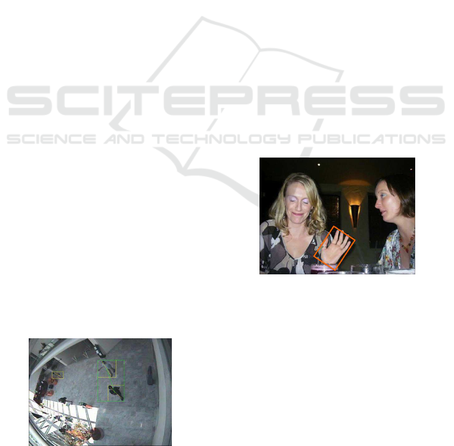
in surveillance applications (figure 1), the detection of
hands (figure 2), objects on a conveyor belt , etc.
Figure 1: Example of rotated appearance of pedestrians
(from CAVIAR dataset (CAVIAR, 2003)).
Rotation gives an extra difficulty to cope with in
object detection, which greatly enlarges the searching
space for our object. The classic solution is to rerun
Figure 2: Rotated hand relative to body (from (Mittal et al.,
2011)).
an object detector on a set of rotated versions of the
input image. Needless to say is that this is far from
computationally efficient. In this paper we propose
a technique to tackle this problem in two steps. We
train multiple models, each covering a specific orien-
tation of the object. Secondly, we create a rotation
map, which predicts at which orientation the object
could be found. This allows us to limit the amount of
models we evaluate at each location, as thus the com-
putational complexity, with a minimum in accuracy
loss. This paper is structured as follows, in section 2
we give an overview of the existing literature about
object detection and rotation invariance, in section 3
we unveil the details of our approach, in section 4 we
give the resuls of the different experiments we have
performed for both accuracy and speed, and finally in
section 5 we end with a conclusion and future work
on this topic.
400
De Smedt F. and Goedemé T..
Fast Rotation Invariant Object Detection with Gradient based Detection Models.
DOI: 10.5220/0005308404000407
In Proceedings of the 10th International Conference on Computer Vision Theory and Applications (VISAPP-2015), pages 400-407
ISBN: 978-989-758-090-1
Copyright
c
2015 SCITEPRESS (Science and Technology Publications, Lda.)
2 RELATED WORK
Object detection is mostly done in two steps. First
a set of features is calculated that emphasize specific
properties of the image. To cope with multiple scales
of the object, the features are calculated for multiple
scales of the image, resulting in a feature pyramid.
The second step is evaluating a pretrained model at
each location of the feature pyramid. When the sim-
ilarity between the model and the features reaches a
certain threshold, that location will be marked as con-
taining the object.
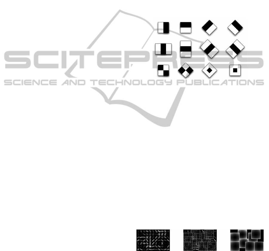
In 2004 (Viola and Jones, 2004) proposed a tech-
nique for face detection using Haar features trained
with Adaboost. The Haar features are simple features
to compare the intensity of pixels over a region. Ex-
amples of such filters are shown in figure 3. By sub-
tracting the dark from the light region, the gradient
information over that region is unveiled. The use of
integral images allows to calculate these features very
fast, independent of the size. The model is formed by
combining a large amount of these features of differ-
ent sizes in a spatial formation.
Later on, in 2005 Dalal and Triggs proposed the
use of Histograms of Oriented Gradients (HOG) for
human detection (Dalal and Triggs, 2005). Hereby,
again, gradients where at the base, although this time
a fine-grained approach is used. The gradients are
calculated for each pixel to its direct neighbors, re-
sulting in a gradient vector for each pixel. The gradi-
ent vectors are then assembled per region of 8x8 pix-
els into a histogram. The histogram bins are formed
by grouping pixels with a similar gradient orientation.
The model is formed by a 2D spatial structure of such
histograms.
To improve the accuracy further, we can distin-
guish two approaches. Integral Channel Features
(Doll´ar et al., 2009) enlarges the kind of features
used for the model. Next to gradient information,
also color information is used. For each annotation
10 channels are calculated (6 histogram orientations,
the gradient magnitude and the LUV color channels).
From a random pool of rectangles containing parts of
the calculated channel features, the ones best describ-
ing the object are selected and used for the model.
Also here an integral image is used for speed pur-
poses. In (Benenson et al., 2013) the training choices
for this detector where studied, leading to one of the
most accurate detectors in current literature. Altough
most of these techniques where applied to pedestri-
ans, they can also be very effective in general object
detection, for example (Mathias et al., 2013) uses the
detector proposed in (Benenson et al., 2013) for traffic
scene recognition.
Recently, (Doll´ar et al., 2014) proposed a tech-
nique to speed-up the calculation of the features. This
is a generalised approach of (Doll´ar et al., 2010).
Hereby the features are only calculated on a limited
amount of scales. The scales in between are approxi-
mated from the calculated ones. As an extra contribu-
tion, they propose a detector, coined Agregate Chan-
nel Features (ACF), which limits the feature pool to
pick from to a rigid grid. This allows both very fast
training and evaluation of the detector. This imple-
mentation is publicly available as part of their toolbox
(Doll´ar, 2013). In this paper the ACF detector is used.
Figure 3: Example of haar features (from (Viola and Jones,
2004)).
Another approach to improve the detection perfor-
mance over a rigid model, is to expand the structure
of the model. In (Felzenszwalb et al., 2008), (Felzen-
szwalb et al., 2010) the structure of the HOG-model
is extended with part-models. So the detection of
an object is divided in searching the root-model (as
was done before), representing the object as a whole,
and the search for part-models at twice the resolution,
representing certain parts of the object. By allowing
the position of each part to deviate a little relative to
the position of the root-model, the Deformable Part
Model (DPM) detector allows a certain pose variation.
Figure 4 visualises the DPM-model for a bycicle (root
model at the left, part-models in the middle and al-
lowed position variation for each part at the right). In
(Felzenszwalb et al., 2010) the evaluation speed was
improved by evaluating the models in a cascaded ap-
proach.
Figure 4: Example of a DPM bycicle model (from (Felzen-
szwalb et al., 2008)).
In (Mittal et al., 2011), a DPM-model is used,
amongst other detection techniques, to detect hands
in images. As mentioned before, hands can appeare
at multiple orientations in an image. To solve this
problem, the image is rotated 36 times (steps of 10
FastRotationInvariantObjectDetectionwithGradientbasedDetectionModels
401
degrees, which they stated gave a good balance be-
tween accuracy and speed) and the detector is evalu-
ated on each rotation. Evidently, this approach has a
high computation cost.
To avoid the requirement of evaluating all possible
orientation with a model, we want to determine the
dominant orientation at each location of the image.
Since interest point description algorithms require to
be rotation invariant, we apply the same strategies in
our work. One of the most common known inter-
est point descriptors is SIFT (Lowe, 1999). Hereby
the rotation of the keypoint is determined by a his-
togram of gradient orientations. The orientation with
the highest magnitude is used as the dominant ori-
entation of the feature. A more detailed description
of this approach, including further precautions for ro-
bustness, can be found in the paper. Although SIFT
succeeds in finding rotation invariant interest points,
the calculation of an orientation histogram would be
to computationally expensive, so we will use a faster
alternative.
To exploit orientation information of the image,
we will use the orientation description technique of
SURF (Bay et al., 2008). SURF combines both high
speed and accuracy, by using integral images in com-
bination with Haar features to describe interest points
of an image. Around each interest point, multiple
sample points are selected. The possitions of those
depend on the scale at which the interest point is
found. For each sample point, both a horizontal and
vertical gradient is calculated using Haar features (as
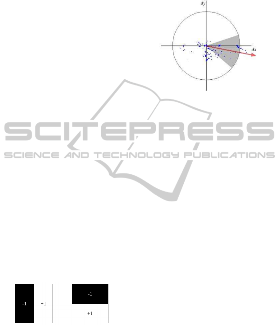
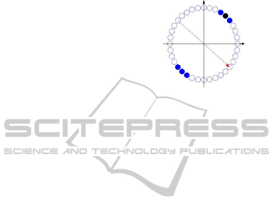
shown in figure 5). To determine the orientation of the
keypoint, each sample point is represented as a point
on a dx-dy-graph, as shown in figure 6. The domi-
nant orientation is found by running the gray area over
the circle in steps of π/12 as a sliding-angle-window,
and summing all vector values (Dx and Dy) for the
points covered by the π/3 wide angle. The maximum
summed vector represents the dominant orientation.
Figure 5: Haar features to extract the horizontal and vertical
gradient as used by SURF (Bay et al., 2008).
3 APPROACH
In this paper we propose a two-step approach to im-
prove object detection speed under rotation with a
Figure 6: How the orientation is determined by SURF (Bay
et al., 2008).
minimal loss in detection accuracy. In the first step,
we transfer part of the computation time to training,
by training a model for each orientation we want to
cover (see section 3.2 for further details). As a sec-
ond contribution, we propose a technique of using a
rotation map which containt orientation information
at each location of the image. This allows for a reduc-
tion of the amount of models evaluated at each loca-
tion. The details are discussed in section 3.3.
To compare with known approaches in literature,
we implemented the approach of (Mittal et al., 2011)
(see section 3.1 for more details), who uses a single
model, which is evaluated on each orientation of the
image. This implementation is used as a comparison
baseline for our approach.
3.1 Rotating the Image
The easiest approach to detect objects under multiple
orientations is by rotating the image multiple times
and apply the object detection algorithm for each ori-
entation. This approach has been performed (amongst
others) by (Mittal et al., 2011) for hand detection us-
ing the DPM-detector.
Although this approach is very intuitive, it comes
with a high computational cost. For each orientation,
the source images has to be rotated, a new feature
pyramid has to be calculated and evaluated. The rota-
tion of the image comes with the issue that each image
has to be rectangular, so black corners appear. Since
these corners have no valuable information, they im-
pose unnecessary processing time.
3.2 Train Rotated Models
To avoid the rotation of the image, we transfer the
processing time to training instead of evaluation, by
training extra models, each covering another orien-
VISAPP2015-InternationalConferenceonComputerVisionTheoryandApplications
402
tation of the model. A similar approach was used by
(Benenson et al., 2012), where multiple models where
trained to cover different scales of the object (avoid-
ing to calculate the features at multiple scales). The
training of models covering the different orientations
does not only avoid the need to rotate the image, but
allows to reuse the feature pyramid of the original im-
age, leading to a tremendous decrease in evaluation
time (as will be discussed in section 4).
A disadvantage of this approach is of course the
extra work to train the models. Some models require
a long training time. For example DPM requires a
training time of ∼7.5 hours per model on a single
core machine. Since our approach is independent of
the detector in use, we use the ACF-object detection
framework instead (Doll´ar, 2013). Since the training
time for a single model is 5 to 6 minutes, depending
on the size of the model, the total training time for all
36 models is around 3.5 hours. This allows for fast
validation of our approach.
For training we used the INRIA pedestrian (train)
dataset (Dalal and Triggs, 2005). This dataset comes
with a large amount of annotated images of pedestri-
ans and images that can be used as negatives. To train
a rotated model, we simply rotate the annotated im-
ages and alter the annotations to a bounding box sur-
rounding the rotated object. To improve the detection
accuracy of the model, a mirrored version of the an-
notation is used. Evidently, a mirrored version of the
annotation can only be used if the object is symetric
(such as pedestrians).
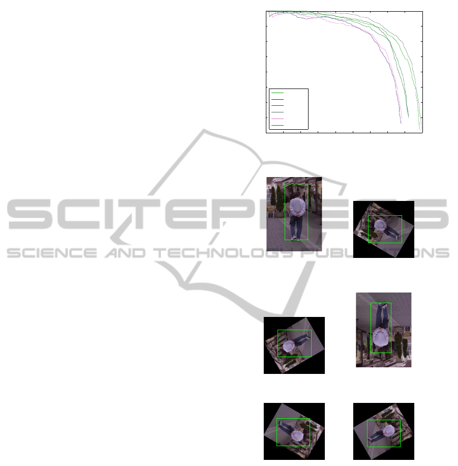
Since we have to use a rectangular model, the
models for a rotated appearance do include back-
ground clutter instead of a rectangles that fits closely
around the object. Altough ACF selects the location
of the features of interest itself, we still observe a cer-
tain accuracy loss by models with more background
clutter, as can be seen in figure 7. We suspect this
loss is due to the default Non-Maximum-Suppression
we use (pruning detections with an overlap of more as
50%). If annotations of the two detected object over-
lap more as 50% it becomes impossible to detect them
both, since the resulting detection windows will be
pruned by the NMS algorithm. The larger the bound-
ing box of the model (caused by extra background
clutter), the higher the chance of this happening. De-
tections of the models used for the accuracy curve (for
the same rotated annotation) are shown in figure 8.
3.3 Retrieving Orientation Information
In the previous section we described how we can op-
timise the evaluation process of rotation invariant ob-
ject detection by training a whole set of models. As
0 0.1 0.2 0.3 0.4 0.5 0.6 0.7 0.8 0.9
0.2
0.3
0.4
0.5
0.6
0.7
0.8
0.9
1
Recall
Precision
Accuracy of rotated models
Angle 0
Angle 60
Angle 120
Angle 180
Angle 240
Angle 300
Figure 7: Accuracy of trained models to cope with rotation.
17.99
15.62
(a) no rotation (b) 60 degrees rotation
23.23
23.06
(c) 120 degrees rotation (d) 180 degrees rotation
23.08
18.04
(c) 240 degrees rotation (d) 300 degrees rotation
Figure 8: The same object under rotation detected by differ-
ent detector models.
can be seen in section 4, this is very beneficial for
speed. In this section we go a step further. For each
position in the image we determine the most proba-
ble orientation the object would be in, by deriving the
dominant orientation of the patch. Our experiments
show that for many objects, this dominant orientation
rotates along with rotating objects. For example by
pedestrians it is perpendicular with the symetry axis.
This allows us to limit the amount of models to run at
each location.
FastRotationInvariantObjectDetectionwithGradientbasedDetectionModels
403
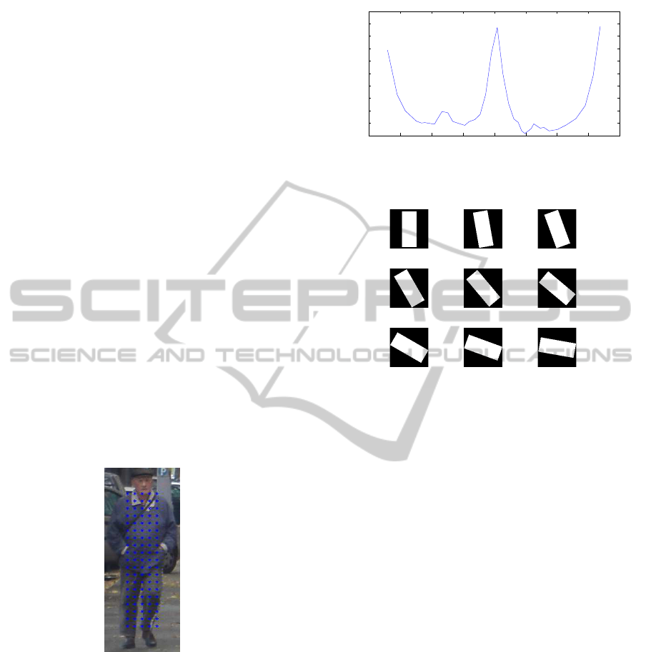
3.3.1 Haar Sample Points
The method to find the dominant orientation is in-
spired by the SURF algorithm. To determine the most
probable orientation to look for the model, we create
a grid of sample points around our evaluation point.
Figure 9 visualises the position of the sample points
on the pedestrian. Here we use a grid of 5 by 19
sample points, evenly distributed. We take the dis-
tance between sample points equal to the stride of the
detector (4px). At each sample point we evaluate a
horizontal and vertical Haar wavelet, as shown in fig-
ure 3, to extract the local gradient vector. The size of
the wavelet is two times the distance between sample
points (so 8px). The use of a sliding-angle-window,
as used by SURF, returns the dominant orientation
for the object. In figure 10, we visualised the average
(normalised) vector magnitude for the pedestrians in
the INRIA trainingset, as we loop over the orienta-
tions. As we can see, we have two dominant orienta-
tions, one around 0 degrees, and one around 180 de-
grees. This can be explained, since the opposite sides
of an object will result in equal but opposite gradi-
ent orientations. We use a 10 degree angle-window
(in contrast to the 60 degrees used by SURF). As will
be explained in subsection 3.3.2, we cope with unbal-
anced aspect ratios by using filters, each covering a
10 degree angle.
Figure 9: Location of the sample points on an annotation.
3.3.2 Handling Unbalanced Aspect Ratios
The technique of using sample points is inspired by
the orientation finding of SURF, where it is used for
a circular region. Because the approach we present
in this paper must work for the detection of arbitrary
objects, this region must be equal to the bounding
box of such an object. Therefor we should determine
the dominant orientation for multiple possible orien-
tations of the model. Figure 11 shows the orientations
we will evaluate in the first (and third) quadrant. If
we follow the basic SURF approach, as explained in
−200 −150 −100 −50 0 50 100 150 200
0.1
0.15
0.2
0.25
0.3
0.35
0.4
0.45
0.5
0.55
0.6
Maximum magnutude over the orientations
Angle
Normalised magnitude
Figure 10: Response at different angles of the magnitude
for upright pedestrians.
0/180 degrees rotation 10/190 degrees rotation 20/200 degrees rotation
30/210 degrees rotation 40/220 degrees rotation 50/230 degrees rotation
60/240 degrees rotation 70/250 degrees rotation 80/260 degrees rotation
Figure 11: Orientations to evaluate in the first (and third)
quadrant.
section 3.3.1, we would have to create a curve similar
to figure 10 for each filter.
Since the full evaluation of all orientations would
cost 36 times the calculation time of a single orienta-
tion, we need to come up with an improved approach.
Based on figure 10, we can state that we are only in-
terested in an orientation if the dominant gradient lies
at the same orientation as the filter (we consider the
filter for the upright position as 0 degrees, altought
the dominant orientation lies perpendicular). There-
fore, we can limit the calculations by using only sam-
ple points inside the filter boundaries, that also has
an orientation that matches the relative orientation of
the filter. Each filter will contribute a single gradient
magnitude for its own orientation (and the inverse).
By searching for the maximum gradient magnitude
over all the filters responses, we can determine the
dominant orientation at a single evaluation point.
The positions of the sample points for a rotated
filter could be determined by just projecting the coor-
dinates of the original filter to the rotated one. This
imposes that we have to evaluate (5x19)x18 = 1710
sample points to figure out the orientation at a single
location. For faster processing speed, we restrict the
positions of the sample points under rotation to the
nearest sample point on a regular grid of 4px. This
limits the amount of sample points necessary for a
VISAPP2015-InternationalConferenceonComputerVisionTheoryandApplications
404
single evaluation point to 301, since a lot of them are
also part of other filters.
For our rotation map, we have to determine the
orientation at each evaluation point. Each sample
point contributes to multiple evaluation point, due to
the sliding window that always overlaps with the pre-
vious positions. Because the stride is equal to the dis-
tance between sample points, we can determine be-
forehand to which evaluation points a sample point
will contribute. This allows us to create a map that
stores the relative position of the sample points that
contribute to an evaluation point based on its orienta-
tion (which defines the filter it is part of).
Instead of reading all the needed sample points for
each evaluation point, we turn around the process. We
loop over the grid of sample points, and for each sam-
ple point we determine its orientation. By using the
map of relative positions, we know to which evalua-
tion points each sample point contributes. This way
each sample point is only read once, and the amount
of contributions per sample points is limited due to
the restriction of orientation.
3.3.3 Approximating Nearby Rotation Maps
Although our optimised strategy for each scale-space
layer (single resize of the original image), the calcu-
lation of the rotation map still requires a lot of pro-
cessing time compared to model evaluation (which is
shown in section 4). To even further speedup the pro-
cess, we can, just as been done for the features, also
approximate rotation maps from nearby scales. The
calculation of the rotation maps over all scales can be
divided in the ones who are calculated based on the
integral image of a scale-space layer, and the ones we
will approximate using nearest neighbour. The ap-
proximation of a rotationmap is faster as to calculate
it from scratch, but the accuracy is proportional to the
correctness. This is discussed in section 4.
3.3.4 Exploiting the Rotationmap for Rotated
Object Detection
With the help of the rotation map, we now have a
thorough idea at which orientation to search for the
object at each location. This help to reduce the num-
ber of rotated object detection models we evaluate on
that location. The model we should always evaluate
is the one proposed by the orientation map. For fur-
ther model selection, we rely on the curve in figure 10,
where we can observe a consistent second peak on the
inverse orientation. Next to that we want to create an
invariance for small mistakes and also run the models
neighbouring our previous selections. This results in
6 from the 36 models to run.
Figure 12: Model selection based on dominant orientation.
In figure 12, the model selection is visualised
when the dominant orientation lies at 320 degrees.
The filter used for this will be oriented perpendicu-
lar (marked in black). As mentioned before, we will
also evaluate the neighbouring models, and the model
at the inverse orientation (all marked in blue).
4 EXPERIMENTS
In this section we will discuss the results of our ap-
proach, both on speed and accuracy. Herefor we
use images from the INRIA pedestrian (test) dataset.
Each image is rotated in steps of 10 degrees. We made
three datasets, each containing a random selection of
1800 images evenly distributed over the orientations.
These 3 datasets are both used for the evaluation of
accuracy and speed.
Below we will refer to the impelemtation decribed
in subsection 3.1 as Rotate, to the implementation of
subsection 3.2 as Multimodel and to the implementa-
tion descibed in subsection 3.3.4 as approx, where the
trailing number states the amount of approximation
used (2 means that 1/2 layers are really calculated, 4
means that 1/4 orientation maps are really calculated
and 8 states that only 1/8 of the layers is really calcu-
lated).
4.1 Accuracy
In order to measure the accuracy, we evaluated the 3
datasets separately by using each of our techniques.
In figure 13 we compare the rotation strategies we
use. As we can observe, the use of multiple models
on the same image comes with a small performance
loss. This is an issue we could expect, since the accu-
racy of the models is also not equal (as seen in figure
7). A more advanced NMS-approach, which takes the
FastRotationInvariantObjectDetectionwithGradientbasedDetectionModels
405
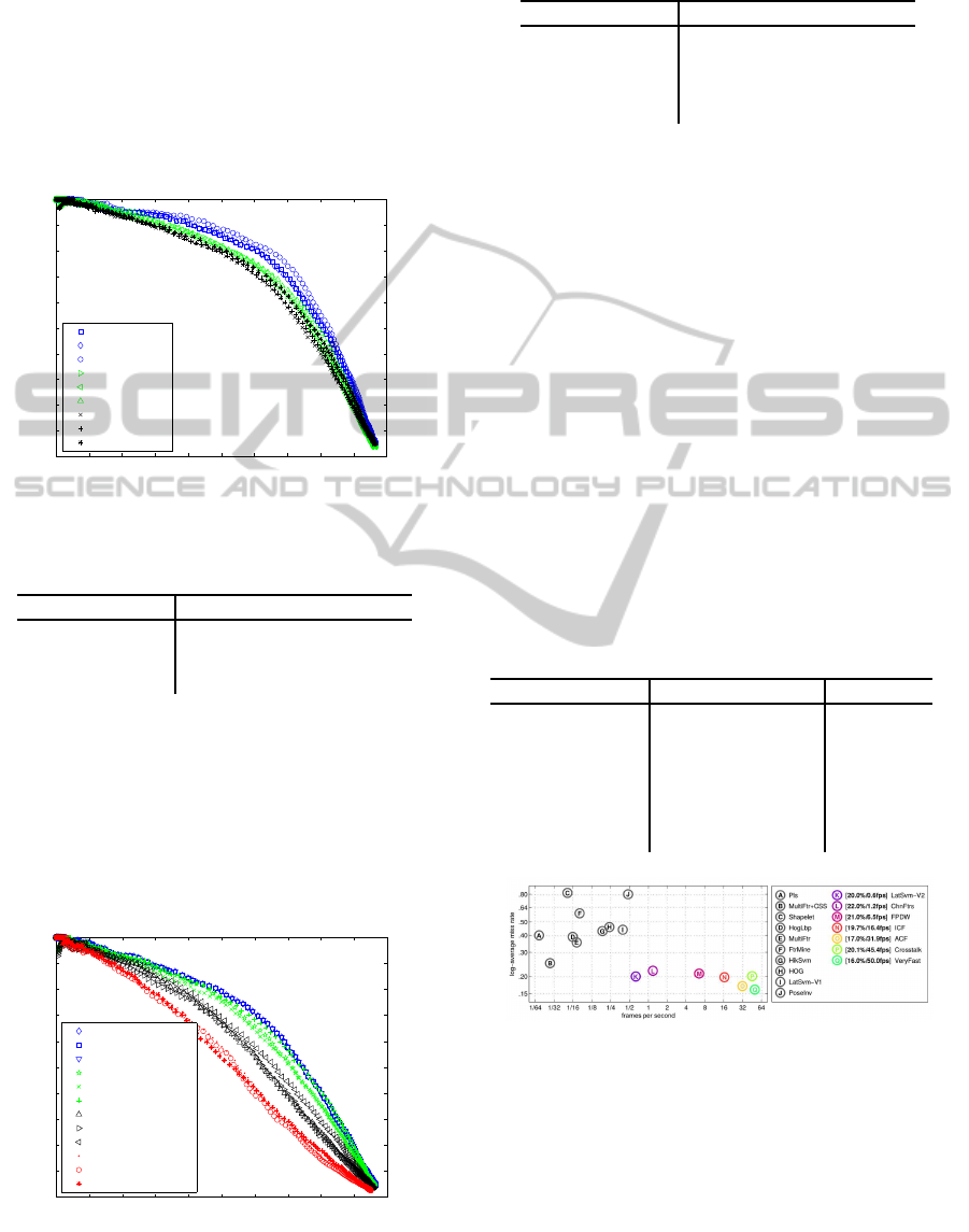
actual location of the object inside the model into ac-
count, could probably make up this gap, but this will
be future work. We also compare with the approach
of using a rotation map to predict the orientation.
Also here we see a performance loss compared with
the multimodel approach, since the smart-approach is
only a reduced version of the multimodel-approach.
The Mean Average Precision of these techniques can
be seen in table 1.
0 0.1 0.2 0.3 0.4 0.5 0.6 0.7 0.8 0.9 1
0
0.1
0.2
0.3
0.4
0.5
0.6
0.7
0.8
0.9
1
Recall
Precision
Accuracy comparison between rotation strategies
Rotate set1
Rotate set2
Rotate set3
Multimodel set1
Multimodel set2
Multimodel set3
Smart set1
Smart set2
Smart set3
Figure 13: The performance of different rotation strategies.
Table 1: Mean Average Precision of rotation strategies over
the 3 datasets.
Technique Mean Average Precision
Rotate 77,7%
Multimodel 74,9%
Smart approx 1
74,1%
In figure 14 we give an overview of the accuracy
that comes with approximating the rotation map in-
stead of calculating it. As we can see, the accuracy
of the rotation map is sensitive to the use of approx-
imation. A more advanced approximation method as
nearest neighbour could bring help here. The Mean
Average Precision over the 3 datasets of the approxi-
mation levels is shown in table 2.
0 0.1 0.2 0.3 0.4 0.5 0.6 0.7 0.8 0.9 1
0
0.1
0.2
0.3
0.4
0.5
0.6
0.7
0.8
0.9
1
Recall
Precision
Accuracy comparison between levels of approximmation
Smart no approx set1
Smart no−approx set2
Smart no−approx set3
Smart 2−approx set1
Smart 2−approx set2
Smart 2−approx set3
Smart 4−approx set1
Smart 4−approx set2
Smart 4−approx set3
Smart 8−approx set1
Smart 8−approx set2
Smart 8−approx set3
Figure 14: The preformance compared between different
amount of approximation.
Table 2: Mean Average Precision of approximation levels
over the 3 datasets.
Approximation Mean Average Precision
Smart approx 1 74.1%
Smart approx 2
70.1%
Smart approx 4 64%
Smart approx 8
55.6%
4.2 Speed
In the first place we are interested in the evaluation
speed of the different approaches (table 3). As we can
see, the use of multiple models pays off. The process-
ing speed is more as 8 times faster as evaluate each
rotation with a single model, and as can be seen in
table 1, this only comes with a minimal loss in ac-
curacy. The speed improvement of using Smart ap-
prox 1 over Multimodel is not that big, but we have to
keep in mind that we are using one of the most opti-
mised detection approaches available for CPU, as can
be seen in figure 15. With no doubt, using a rotation
map has a greater impact when a more complex model
is necessary (such as DPM). We can also see that the
approximation of the rotationmap leads to a very high
speed improvement, but the accuracy loss that comes
with it is too high for practical use (see section 4.1).
Table 3: Comparing the processing speeds of the different
approaches.
Technique Evaluation Speed Speed-up
Rotate 0.184 FPS 1 X
Multimodel
1.5 FPS 8.12 X
Smart approx 1 1.51 FPS 8.20 X
Smart approx 2
1.83 FPS 9.98 X
Smart approx 4 2.11 FPS 11.51 X
Smart approx 8 2.24 FPS 12.18 X
Figure 15: Comparison of speed and accuracy of detectors
(from (Doll´ar et al., 2014)).
To better understand the gain in evaluation time,
we visualised the relative time that is spend at each
part of the evaluation pipeline. As can be seen in fig-
ure 16, the amount of time spend at calculating the
feature pyramid for each rotation of the image forms
the mean bottleneck of Rotate. This issue is com-
pletely avoided in Multimodel, where, as could be ex-
pected, the main calculation time is performed dur-
VISAPP2015-InternationalConferenceonComputerVisionTheoryandApplications
406

ing model evaluation. This proves that the optimised
evaluation process of this detector is very beneficial
for the total evaluation time. As we also could ob-
serve in the speed results of table 3, the calculation of
the rotation map is very computation intensive com-
pared to the other parts of the evaluation pipeline. An
improvement in its evaluation speed would be of great
impact on the speed-up it can attain.
Figure 16: The deviation of calculation time between rota-
tion approaches.
5 CONCLUSION
5.1 Conclusion
In this paper we propose a two-step approach to im-
prove the processing speed of object detection under
rotation. As a first step we trained multiple models to
cover all needed orientations. This allows to eliminate
the need to rotate the image, and allows to reuse the
feature pyramid for all models. Next to that we use
sample points to extract orientation information over
the image. This allows us to reduce the number of
models that have to be evaluated at each location. We
used the ACF-detection frameworkfor its fast training
and evaluation speed and aquired still a speed-up by
using a rotation map. We compare to the baseline of
evaluating multiple rotations of the image, and aquire
a speed-up of 8.2 times, while maintaining high accu-
racy.
5.2 Future Work
As a follow-up of this work, we plan to test our ap-
proach with other object detection algorithms, such as
DPM. Next to that we will try to eliminate the accu-
racy loss by improving the NMS-algorithm and work
on a better approximation technique for the rotation
map. We also plan to apply the rotation invariance in
multiple cases such as surveillance applications and
hand detection.
REFERENCES
Bay, H., Ess, A., Tuytelaars, T., and Van Gool, L. (2008).
Speeded-up robust features (surf). Comput. Vis. Image
Underst., 110(3):346–359.
Benenson, R., Mathias, M., Timofte, R., and Van Gool, L.
(2012). Pedestrian detection at 100 frames per second.
In Computer Vision and Pattern Recognition (CVPR),
2012 IEEE Conference on, pages 2903–2910. IEEE.
Benenson, R., Mathias, M., Tuytelaars, T., and Van Gool, L.
(2013). Seeking the strongest rigid detector. In Com-
puter Vision and Pattern Recognition (CVPR), 2013
IEEE Conference on, pages 3666–3673. IEEE.
CAVIAR (2003). Caviar: context aware vision using image-
based active recognition.
Dalal, N. and Triggs, B. (2005). Histograms of oriented gra-
dients for human detection. In Computer Vision and
Pattern Recognition, 2005. CVPR 2005. IEEE Com-
puter Society Conference on, volume 1, pages 886–
893. IEEE.
De Smedt, F., Van Beeck, K., Tuytelaars, T., and Goedem´e,
T. (2013). Pedestrian detection at warp speed: Ex-
ceeding 500 detections per second. In Computer Vi-
sion and Pattern Recognition Workshops (CVPRW),
2013 IEEE Conference on, pages 622–628. IEEE.
Doll´ar, P. (2013). Piotrs image and video matlab toolbox
(pmt). Software available at: http://vision. ucsd. edu/˜
pdollar/toolbox/doc/index. html.
Doll´ar, P., Appel, R., Belongie, S., and Perona, P. (2014).
Fast feature pyramids for object detection. IEEE
Trans. Pattern Anal. Mach. Intell., 36(8):1532–1545.
Doll´ar, P., Belongie, S., and Perona, P. (2010). The fastest
pedestrian detector in the west. In BMVC.
Doll´ar, P., Tu, Z., Perona, P., and Belongie, S. (2009). Inte-
gral channel features. In BMVC, volume 2, page 5.
Felzenszwalb, P., McAllester, D., and Ramanan, D. (2008).
A discriminatively trained, multiscale, deformable
part model. In Computer Vision and Pattern Recog-
nition, 2008. CVPR 2008. IEEE Conference on, pages
1–8. IEEE.
Felzenszwalb, P. F., Girshick, R. B., and McAllester, D.
(2010). Cascade object detection with deformable part
models. In Computer vision and pattern recognition
(CVPR), 2010 IEEE conference on, pages 2241–2248.
IEEE.
Lowe, D. G. (1999). Object recognition from local scale-
invariant features. In Computer vision, 1999. The pro-
ceedings of the seventh IEEE international conference
on, volume 2, pages 1150–1157. Ieee.
Mathias, M., Timofte, R., Benenson, R., and Van Gool, L.
(2013). Traffic sign recognitionhow far are we from
the solution? In Neural Networks (IJCNN), The 2013
International Joint Conference on, pages 1–8. IEEE.
Mittal, A., Zisserman, A., and Torr, P. H. (2011). Hand
detection using multiple proposals. In BMVC, pages
1–11. Citeseer.
Viola, P. and Jones, M. J. (2004). Robust real-time face
detection. International journal of computer vision,
57(2):137–154.
FastRotationInvariantObjectDetectionwithGradientbasedDetectionModels
407
