Video Segmentation via a Gaussian Switch Background Model and

Higher Order Markov Random Fields

Martin Radolko and Enrico Gutzeit

Fraunhofer Institute for Computer Research IGD, 18059 Rostock, Germany

Keywords:

Image Segmentation, Background Substraction, Belief Propagation, Otsu’s Method, Markov Random Fields.

Abstract:

Foreground-background segmentation in videos is an important low-level task needed for many different ap-

plications in computer vision. Therefore, a great variety of different algorithms have been proposed to deal

with this problem, however none can deliver satisfactory results in all circumstances. Our approach combines

an efﬁcent novel Background Substraction algorithm with a higher order Markov Random Field (MRF) which

can model the spatial relations between the pixels of an image far better than a simple pairwise MRF used in

most of the state of the art methods. Afterwards, a runtime optimized Belief Propagation algorithm is used

to compute an enhanced segmentation based on this model. Lastly, a local between Class Variance method is

combined with this to enrich the data from the Background Substraction. To evaluate the results the difﬁcult

Wallﬂower data set is used.

1 INTRODUCTION

Nowadays Vision Systems are used in many ﬁelds

of applications such as surveillance, industrial au-

tomation, transportation or inspection. In the last

decades Background Substraction has become a valu-

able source of low level visual information. It can de-

tect arbitrary objects in almost any scene, as long as

they are in motion. This information can afterwards

be used for all kinds of high-level vision tasks.

In order to gather the aforementioned data the

background for each individual scene has to be mod-

elled. The creation of this model is not a trivial task

and associated with many difﬁculties like changes in

the lightning conditions, moving background objects

(swaying trees), shadows or a changing background.

To cope with all these requirements a great number

of different approaches have been deployed. Some

use Subspace Learning Models like LDA (Kim et al.,

2007), INMF (Bucak et al., 2007) or PCA (Marghes

et al., 2012) to generate a background model. Other

prominent methods adopt techniques like Kalman Fil-

ters (Cinar and Principe, 2011), SVMs (Lin et al.,

2002) or histograms (Zhang et al., 2009) to cope with

these problems.

However, most of the current algorithms model

each background pixel as a Gaussian Distribution.

This is justiﬁed by the fact that the intensity of a pixel

in a completely static scene will vary according to a

Normal distritution N (µ,σ

) due to the measurement

errors inherent in every camera system. With this in-

formation, a threshold per pixel can be easily created

to distinguish between foreground and background.

There are approaches which use just one Normal

Distribution per pixel (Wren et al., 1997), algorithms

which use a Mixture of Gaussians (Stauffer and Grim-

son, 1999; Setiawan et al., 2006) or Gaussian-Kernel

based methods (Elgammal et al., 2000) to model the

background. Methods which use a Mixture of Gaus-

sians (MoG) produce in most cases better results than

the Single Gaussian (SG) algorithms, but also have

some disadvantages. One is a higher memory usage

and another the need to be tuned for the right amount

of Gaussians.

A shared drawback of all Background Substrac-

tion approaches is that they do not incorporate the

spatial informations about the scene in the model,

although natural images are commonly assumed to

be very smooth. To use this assumption to improve

the segmentation derived from the Background Sub-

straction different strategies have been applied. In

(Toyama et al., 1999) a simple approach is used which

discards all connected regions containing less than a

certain amount of pixels. A more complex approach

is used in (Y. Wang and Wu, 2006) where a Condi-

tional Random Field models the neighbourhood rela-

tions of the pixels. Graph Cuts are used in (Boykov

and Funka-Lea, 2006) and to represent the spatial in-

537

Radolko M. and Gutzeit E..

Video Segmentation via a Gaussian Switch Background Model and Higher Order Markov Random Fields.

DOI: 10.5220/0005308505370544

In Proceedings of the 10th International Conference on Computer Vision Theory and Applications (VISAPP-2015), pages 537-544

ISBN: 978-989-758-089-5

 2015 SCITEPRESS (Science and Technology Publications, Lda.)

formation in all dimension in a Subspace Model a

Tensor was applied (Li et al., 2008).

The most frequently utilized method for this prob-

lem is a MRF which models the relations via an undi-

rected graph. The most likely overall state of the

model (maximum a posteriori probability - MAP) will

correspond with a good segmentation if the underly-

ing data (a probability map) is adequate. Since it is

NP-hard to compute the MAP for a cyclic MRF, there

exists several methods to approximate the best solu-

tion. In (Xu et al., 2005) Gibbs-Sampling is combined

with simulated annealing, (Sun et al., 2012) applies

a Branch and Bound algorithm and (Yedidia et al.,

2003) utilises a Belief Propagation method to get a

good approximation of the MAP.

Building on this, a new method composed of three

parts is developed. First, a new Background Substrac-

tion algorithm will be proposed which uses exactly

two Gaussians and thereby eliminates most of the dis-

advantages of the MoG approaches, but nonetheless

generates state of the art results. Secondly, a higher

order MRF with a variable neighbourhood is created

to model the spatial relations of the objects in the

scene. A Belief Propagation algorithm is used to de-

rive a suitable approximation of the MAP. Lastly, a

component was added which inﬂuences the segmen-

tation to maximize the between-class variance. The

basic idea was ﬁrst proposed in (Otsu, 1979) and

is widely appreciated since then (Liao et al., 2011;

Huang et al., 2001). Here, the approach is used in

a combination with the Belief Propagation algorithm

so that the between class variance is optimized during

the iterations as well.

2 HIGHER ORDER MARKOV

RANDOM FIELDS

The MRF is a well established and widely used statis-

tical model which can describe the dependencies be-

tween various random variables. It originates from

the works of Ising on ferromagnetism (Ising, 1925)

but was since extended and adopted to a large number

of different problems.

A small example of a MRF represented as a graph

can be seen in Figure 1. The random variables are

depicted as circles and the edges show the dependen-

cies between them. This easy and graphical way of

modeling the relations between random variables can

be useful in a great variety of applications, one ex-

ample are the spatial relations between pixels in an

image. In this case every pixel is represented by one

random variable for which the state is unknown and

which has dependencies on all neighbouring pixels.

Figure 1: A graphical depiction of a small MRF.

Thereby, the state of a random variable could indi-

cate if the corresponding pixel is in the foreground

of the image, denote the optical ﬂow at that point or

any other information which can be deduced from the

data.

A crucial point for this is the selected neighbourhood

system. A small system like the von Neumann neigh-

bourhood might be unable to model all the complexity

of the relations and bigger systems will soon create

models which are unmanageable. For computer vi-

sion algorithms the von Neumann neighbourhood is

almost always chosen because it will create a pair-

wise MRF. These MRF have the advantage that they

only have cliques of one or two nodes which makes

the computation much easier.

The computational difﬁculties derive from the fact

that in every clique all members will be inﬂuenced

from all the others. To deduce an approximate so-

lution of the MAP a Belief Propagation algorithm

will compute messages from every clique to all of its

members. This means that in Figure 1 node E will

receive one message depending only on A (E and A

are a clique), one depending only on B but also a third

message depending on both of them (A, E and B are

a clique). For bigger neighbourhoods each node can

be in tens or even hundreds of different cliques which

will make the computation and storage of all the mes-

sages nearly impossible.

In the Moore neighbourhood, which is the next

bigger neighbourhood system occasionally used for

images, every node is already a member in 24 cliques.

Also, it has to be noted that there is not just one mes-

sage from every clique to each member but one mes-

sage for every possible state the whole clique can be

in. To reduce this heavy computational load there will

be two techniques introduced in section 3.2 which

will make it possible to compute good approxima-

tions of the MAP even for advanced neighbourhood

systems.

Until now the proposed MRF only models the spa-

tial relationship of the pixels. To generate good seg-

mentations the information given by the image also

have to be included into the model. In the proposed

method this will be a value generated by the Back-

ground Substraction method denoting the probabil-

ity of a pixel being in the background. To include

this information, a second node with a ﬁxed/known

VISAPP2015-InternationalConferenceonComputerVisionTheoryandApplications

538

state will be created for every pixel. This new node

is called an evidence node because it represents given

information in the model. The others are called hid-

den nodes since they indicate an unknown state of the

system which shall be deduced. Every evidence node

will inﬂuence only the corresponding hidden node

and in a way that it will more likely attain the state

favoured by the given data. An example of a MRF

model with a Moore Neighbourhood can be seen in

Figure 2.

Figure 2: The evidence nodes are drawn as small dark cir-

cles. Each is connected with one edge to the corresponding

hidden node. For two hidden nodes the edges to the other

neighbouring hidden nodes are also drawn.

3 OUR APPROACH

Our approach consists of three main steps.

• First, a novel efﬁcient Gaussian Switch Model

is used to create an approximation of the back-

ground which is then subtracted from every new

frame to create a ﬁrst segmentation.

• A MRF is used in the second step to model the

spatial relations between the pixels. Unlike many

other approaches, a MRF of higher order is used

here to reproduce the relations between different

pixels in the MRF more precisely.

• In the last step, a local version of Otsu’s Method is

added to optimize the data generated by the Back-

ground Substraction. These changes will inﬂu-

ence the Belief Propagation, so that the resulting

segmentation has a high local between Class Vari-

ance which will further improve the outcomes.

3.1 The Gaussian Switch Model

As justiﬁed previously, Gaussian distributions are

used to model the colour of each pixel. Instead of

using a batch method, which will save the last n pic-

tures and generate a background model from these,

the Gaussians are updated with every new frame to

save memory and computing power. Thereby, the al-

gorithm gives the new samples automatically a higher

weight than old samples and thus even improves the

results in comparison to the batch method. For ev-

ery Gaussian, the mean µ and variance σ

have to

be stored. The mean is initiated with the pixel value

taken from the ﬁrst frame of the video stream and the

variance is set to a predeﬁned value. Afterwards, they

are updated in the following way

t+1

= α µ

+ (1 −α) v

, (1)

(σ

t+1

)

= α σ

+ (1 −α)(µ

− v

)

. (2)

The variable α ∈ [0,1] controls the update rate and v

is the pixel value taken from the t-th frame. In the

rest of the paper the index t will be omitted because

all variables are taken from the same frame.

With these formulas, the Gaussian distribution of

a background pixel can be modelled very precise and

efﬁcient. Nevertheless, one problem is that the dis-

tribution becomes erroneously when a foreground ob-

ject is visible. To overcome this problem, the back-

ground Gaussian N (µ

,(σ

)

) is created which will

only get updated when the new pixel is classiﬁed as

background. This results in a much more resilient

background model but has two inherent problems.

The ﬁrst issue are objects in motion visible in the ﬁrst

frame because the real background in this area would

never get included into the model. The other problem

are foreground objects that become background (e.g.

a car that parks), because they will never get included

into the background model. To eliminate these errors

an overall Gaussian N (µ

,(σ

)

) is needed which

will be updated with every new frame.

If this overall Gaussian has a small variance but a

different mean than the background Gaussian, a fore-

ground object was visible and immobile for a long pe-

riod of time. This foreground object should therefore

become a part of the background model. To achieve

this, the mean and variance of the background Gaus-

sian are switched to the overall Gaussian’s values.

Now, one intensity value per pixel can be modelled

in this way but most videostreams today are not in

grayscale and consequently have three colour values

for each pixel. To use these additional data a special

colour space is applied which normalises the differ-

ent intensities in respect to the illumination (Li et al.,

2008). Let R, G and B be the given values for a sin-

gle pixel in the standard RGB colour space, then these

will be transformed into the three new image channels

I = R + B + G,

R = R/I,

B = B/I.

VideoSegmentationviaaGaussianSwitchBackgroundModelandHigherOrderMarkovRandomFields

539

Afterwards the intensity I is normalized, so that all

values are in the range of [0, 1]. The colour informa-

tion stored in

R and

B are normalised with the inten-

sity and will thus not be altered by small or medium

changes in the lighnting conditions. This is used to

avoid the detection of shadows as foreground.

For each of these three values an independent

Gaussian Switch Model (GSM) has to be applied. To

decide whether a pixel matches the background model

the values for each channel will be separately com-

pared to the corresponding GSM. Let p

be the new

value for a pixel, it is classiﬁed as matching the back-

ground model if the following inequality is satisﬁed:

− µ

)

< max(β · (σ

)

,0.001). (3)

The maximum is used because the variance could ap-

proach near zero values, especially since only match-

ing values are included into the background model.

The parameter β can control the range of values which

are still classiﬁed as “matching the model”. This use

of the variance provided the algorithm with a pixel-

wise adaptive threshold.

To get a decision for a single pixel as a whole

a voting procedure is chosen. If for a single pixel

equation (3) is satisﬁed for atleast two channels, then

the pixel is marked as background, otherwise as fore-

ground. Thereby, the colour information can overrule

the brightness information and hence shadows should

not be detected as foreground.

In (Toyama et al., 1999) a method is proposed

which takes global changes in the lightning condition

into account, for example when a cloud is blocking

the sun and makes the whole scene darker. These

events often result in the classiﬁcation of almost the

whole scene as foreground and afterwards it takes the

model a long time to adapt to the new conditions. To

improve this behaviour, the algorithm will check in

every new frame if more than 75% of the pixels are

classiﬁed as foreground, if only the intensity channel

is taken into consideration. Should this be the case

the update rate α is set to 0.5 to increase the adaption

speed of the model drastically.

3.2 The Markov Random Field

In the next step the result from the Background Sub-

straction algorithm will be optimized by correcting

small areas with false detections to get contiguous

foreground and background regions. To achieve this

the MRF described in section 2 is used. It can model

the spatial relations between single pixels and hence

forces the segmentation to be locally coherent.

The neighbourhood system is the most important

part of a MRF. Here a Generalized Moore Neighbour-

hood (GMN) is used to ensure the homogeneity of

the MRF and because it can be easily changed in size.

The normal Moore Neighbourhood is shown in Figure

2 for two different nodes. For a node N this neigh-

bourhood system is deﬁned by a three times three

square of nodes with N in the center of it. All nodes

of the square are then neighbours of N. The ﬁrst or-

der GMN uses a 5 × 5 square instead of a 3 × 3 one,

the second order GMN then enlarges this to a 7 × 7

square and so forth. Hereby, the number of cliques

will increase radically with the order of the GMN.

As input the MRF needs in principle two values

for each pixel, one should indicate the probability of

the pixel for being in the foreground and the other the

probability of being in the background. These data is

needed for the evidence nodes, so that they can rep-

resent the result of the Background Substraction al-

gorithm. Here just one value w

is used, which is the

probabilty that the pixel i belongs to the background.

As this value is already normalisied the other proba-

bility can be set to 1 − w

. To calculate w

the voting

algorithm is used again. At the beginning w

is set to

0.9 and then for each of the three channels which does

not match the background model the value is lowered.

For the two colour channels 0.3 are subtracted

in each case and for the intensity channel 0.2 is de-

ducted. By this means the probability will always be

above 50% if at least two of the channels favour the

background and less than 50% otherwise. The colour

channels get an higher weight because a change in the

colour is a better indicator for the pixel being fore-

ground than a change in the intensity.

To eventually compute an approximation of the

MAP a cost function has to be deﬁned which mea-

sures how good a segmentation matches the MRF

model. A function D(i) is needed for the evidence

nodes and shall describe how good a certain state of

the corresponding hidden node matches the data de-

livered from the Background Substraction. In our

case the function for the hidden node i is deﬁned as

follow:

D(i) =



, i is background

1 − w

, i is foreground

(4)

A second set of functions is necessary for the cliques

of hidden nodes. They are named C

, the k indicating

the size of the clique. These functions should rep-

resent the spatial relationship between the pixels and

hence there can be different functions for all possi-

ble clique sizes and spatial arrangements. However,

in this case the beneﬁcial homogenous structure of

the MRF can be exploited. Since all hidden nodes

have the same neighbourhood and a coherent segmen-

tation shall be created everywhere, the functions C

can be the same for all nodes. A small exception are

the boundaries, there the neighbourhood is smaller

VISAPP2015-InternationalConferenceonComputerVisionTheoryandApplications

540

and consequently the number of cliques decreases.

Nonetheless, for the remaining cliques the standard

functions can be applied.

More problematic is the fact that different function

values have to be calculated for every single clique a

node is part of, this increases the complexity of the

model dramatically. To reduce the computational load

only one clique size was chosen to contribute to the

energy function. This simpliﬁcation will drastically

decrease the number of messages which have to be

send later in the Belief Propgation algorithm.

Another way to lessen the computational burden is

the usage of a simple energy function for the remain-

ing cliques. Due to the fact that large homogenous

fore- or background regions are presumed, the func-

tions C

should favour the cases where all nodes in

the clique have the same state. This can be achieved

by returning 0 energy for this case and a positiv static

value for all other cases. Equation (5) gives an exam-

ple for the case k = 4, there h

to h

are the states

of the four different hidden nodes contained in the

clique.

) =



0, h

= h

1, elsewise

(5)

These simpliﬁcations are required, since without

them it would not be feasible to use more than the

Moore Neighbourhood on any picture with a reason-

able resolution. A comparison of the effects of dif-

ferent neighbourhood systems and clique sizes can be

seen in Figure 3 in the result section.

To eventually compute the MAP of the MRF the

respective graph was ﬁrst converted to a factor graph

and then a loopy max-product Belief Propagation was

applied. For details see (Yedidia et al., 2003) and

(Felzenszwalb and Huttenlocher, 2004).

3.3 Using the Between Class Variance

In (Otsu, 1979) a method is described to segment a

picture into two classes by maximizing the variance

between the two classes. This results in an useful

segmentation only under very speciﬁc circumstances.

Namely, when the objects of interest are all similar

among them and different from the background in

colour and brightness. It is obvious that this assump-

tion cannot be made in real life images.

However, in most cases this assumption will hold

if only a small area around a pixel is taken into ac-

count. To use this to improve the segmentation cre-

ated in the ﬁrst two steps, a local between Class Vari-

ance is introduced and coupled with the Belief Prop-

agation to enrich the data taken from the Background

Substraction in each iteration.

A segmentation has to be known ﬁrst to compute

the between Class Variance. For this reason, one is

created after every iteration of the Belief Propagation

algorithm and then for every pixel the average colours

of all background and foreground pixels, but only in

a small square-sized area around this pixel, are cal-

culated. Now the background probability w

will be

increased if the colour of current pixel is closer to the

background average colour and lowered elsewise.

To be more precise, let c

= (c

) and

f g

be the local average colour of the background re-

spectively foreground and c

the colour of the cur-

rent pixel. If kc

− c

< kc

f g

− c

the between

class variance will increase when the current pixel is

classiﬁed as background. If the inequality does not

hold, the pixel should be classiﬁed as foreground to

increase the local between class variance.

However, the classiﬁcation of the current pixel

will not be directly changed according to the between

Class Variance. Instead, the data obtained from the

Background Substraction is altered to reinforce a clas-

siﬁcation which increases the local between Class

Variance in the following iterations. For the pixel i

this is done by computing the value

= γ · (kc

f g

− c

− kc

− c

) (6)

and changing the probability w

accordingly. Gamma

is a factor which controls the impact the Class Vari-

ance will have on the data from the Background Sub-

straction. Now the values p

and p

f g

can be calcu-

lated which represent the new foreground and back-

ground probabilities,

= max(w

+ v

,0.001)

f g

= max((1 − w

) − v

,0.001).

The maximum is required to avoid negativ probabili-

ties. In the next step these values have to be normal-

ized so that p

+ p

f g

= 1 and afterwards the value w

can be replaced by p

This process improves the results but is also com-

putational expensive, especially the calculation of the

average values c

and c

f g

for every pixel in every

iteration for every frame. To reduce the runtime, In-

tegral Images (ﬁrst introduced by (Viola and Jones,

2004)) are used to efﬁciently compute these values in

a static time, independent of the size of the square-

sized area over which these values are averaged. For

every channel two Integral Images have to be created,

one for the background pixels and one which only

adds up the foreground pixels. After calculating these

integral images the actual averages can be obtained by

a simple operation consisting only of three additions.

VideoSegmentationviaaGaussianSwitchBackgroundModelandHigherOrderMarkovRandomFields

541

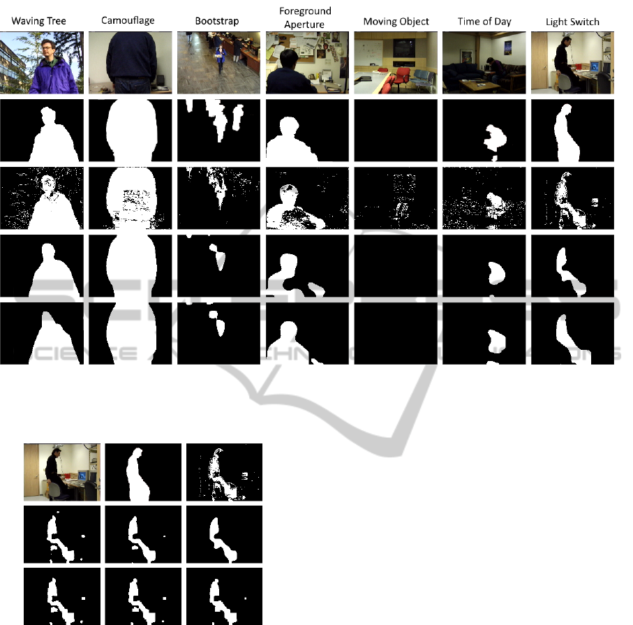
Figure 4: This ﬁgure depicts the results the proposed approach generated for the Wallﬂower data set. The ﬁrst row shows the

images from the videos, the second row the corresponding ground-truth data, the next the results after the GSM algorithm,

the fourth row the results when the GSM is combined with the MRF (without the Between Class Variance) and the last row

shows the results of the ﬁnal algorithm.

Figure 3: The ﬁrst row shows the original picture, the

ground-truth data and the result after the GSM. In the sec-

ond row the results after the smallest clique Belief Propa-

gation algorithm with the Moore Neighbourhood, ﬁrst and

second order GMN are depicted. The last row shows the

same for the maximal clique Belief Propagation.

4 RESULTS

To compare our algorithm with existing methods the

Wallﬂower data set (Toyama et al., 1999) is chosen

because various different methods were already eval-

uated with it. Each of the seven examples depicts one

unique problem of video segmentation which can be

assessed with the provided ground-truth data.

As only one size of cliques is taken into considera-

tion by the Belief Propagation, a comparison between

two algorithms which use different clique sizes is

made. One would only factor in the maximal cliques

and another only the smallest cliques (C

). Both al-

gorithms achieved considerable improvements of the

segmentation delivered by the Background Substrac-

tion and the extracted foreground regions are in gen-

eral smoother if the minimal clique method is used

(see Figure 3). For the ﬁnal results the second or-

der GMN and the algorithm which used the smallest

cliques are applied.

The results for all video sequences and the three

stages of our approach with one set of parameters are

shown in Figure 4. It can be seen that the GSM alone

generates good segmentations but still has many sin-

gle false detections. A good example of this is the

segmentation of the Moving Object scene.

In general, these can be very good eliminated with

the MRF approach and only areas in which whole ob-

jects were not or falsly detected remain as errors (see

Bootstrap or Foreground Aperture). As the results

with the MRF are already quite good, the range of

improvement for the between Class Variance addition

to the Belief Propagation is limited. Nonetheless, it

enhances the overall results considerably, mainly by

expanding the foreground area if the surrounding pix-

VISAPP2015-InternationalConferenceonComputerVisionTheoryandApplications

542

Table 1: The results of different algorithms for the Wallﬂower data set. Each row shows the number of wrongly classiﬁed

pixels for one approach separated in false positives and false negatives.

Algorithm MO ToD LS WT C B FA Total

Single Gaussian FN 0 949 1857 3110 4101 2215 3464

(Wren et al., 1997) FP 0 535 15123 357 2040 92 1290 35133

Mixture of Gaussian (MoG) FN 0 1008 1633 1323 398 1874 2442

(Stauffer and Grimson, 1999) FP 0 20 14169 341 3098 217 530 27053

Kernel Density Estimation FN 0 1298 760 170 238 1755 2413

(Elgammal et al., 2000) FP 0 125 14153 589 3392 993 624 26450

MoG with PSO FN 0 807 1716 43 2386 1551 2392

(White and Shah, 2007) FN 0 6 772 1689 1463 519 572 13916

MoG in improved HLS Color Space FN 0 379 1146 31 188 1647 2327

(Setiawan et al., 2006) FP 0 99 2298 270 467 333 554 9739

MoG with MRF FN 0 47 204 15 16 1060 34

(Schindler and Wang, 2006) FP 0 402 546 311 467 102 604 3808

Gaussian Switch Model (GSM) FN 0 457 1636 244 829 1708 1567

this paper FP 466 641 543 736 164 166 561 9718

GSM with Belief Propagation (BP) FN 0 394 1789 113 208 2064 1686

this paper FP 0 40 289 156 13 3 414 7169

GSM with improved BP FN 0 321 1383 174 246 2081 469

this paper FP 0 199 695 356 66 0 92 6092

Independent Component Analysis FN 0 1199 1557 3372 3054 2560 2721

(Tsai and Lai, 2009) FP 0 0 210 148 43 16 428 15308

Nonnegativ Matrix Factorization FN 0 1282 2822 4525 1491 1734 2438

(Bucak and Gunsel, 2009) FP 0 159 389 7 114 2080 12 17053

Wallﬂower FN 0 961 947 877 229 2025 320

(Toyama et al., 1999) FP 0 25 375 1999 2706 365 649 11478

els have a very similar colour.

An assessment of the results can be seen in Table

1 where the number of pixels which were wrongly

classiﬁed are shown for all videos and many differ-

ent approaches. The upper part shows various meth-

ods which are all using Gaussians for modelling the

background. In the middle the results of our approach

are illustrated and in the lower part are some meth-

ods which use completlely different principles (non-

Gaussian) to model the background.

As the GSM method uses Gaussians for the back-

ground modeling it should be primarily compared to

the Single Gaussian or MoG approaches shown at the

top of the table. Although the GSM uses only two

Gaussians and is therefore not as memory consum-

ing as the MoG methods (which normally are tuned

to ﬁve or more Gaussians), it still does perform bet-

ter than almost all of them. Only one method could

generate better results than the GSM algorithm when

it was combined with the MRF and Otsu’s Method.

5 CONCLUSION

A new and efﬁcient way to model the background of

a video with Gaussians is proposed and linked with a

novel voting mechanism. The updated model is sub-

tracted from every new frame and with a pixelwise

adaptive threshold a segmentation can be created. In a

second step the segmentation was improved by apply-

ing a higher order MRF on the generated data. There

several adaptations were applied to obtain a manage-

able model even with advanced neighbourhood sys-

tems. Lastly, the Belief Propagation algorithm used

to solve the MRF was extended by a process which

would change the underlying probability map based

on a local version of Otsu’s method.

The beneﬁt of the approaches using the MoG

method should theoretically be mainly in cases like

the Waving Tree video, where background objects are

constantly in motion but do not become foreground.

In this case the different backgrounds per pixel can

be speciﬁcally modelled by the different Gaussians of

the MoG. In practice, the GSM algorithm performs

equally good there, although it only models one back-

ground per pixel.

The adaptions made to the MRF to simplify the

calculation of the MAP made it possible to use this

model on a today’s standard PC and still achieve sub-

stantial and reliable improvements of the segmenta-

tion. Furthermore, it is demonstrated that the local

version of Otsu’s Method can alter the segmentation

in a way that it aligns with the borders of the objects

in the given scene. Overall this new approach delivers

state of the art results in this well-studied subject.

VideoSegmentationviaaGaussianSwitchBackgroundModelandHigherOrderMarkovRandomFields

543

REFERENCES

Boykov, Y. and Funka-Lea, G. (2006). Graph cuts and ef-

ﬁcient n-d image segmentation. International Journal

of Computer Vision, 70:109–131.

Bucak, S., Gunsel, B., and Guersoy, O. (2007). Incremental

nonnegative matrix factorization for background mod-

eling in surveillance video. In Signal Processing and

Communications Applications, 2007. SIU 2007. IEEE

15th, pages 1–4.

Bucak, S. S. and Gunsel, B. (2009). Incremental subspace

learning via non-negative matrix factorization. Pattern

Recogn., 42(5):788–797.

Cinar, G. and Principe, J. (2011). Adaptive background esti-

mation using an information theoretic cost for hidden

state estimation. In Neural Networks (IJCNN), The

2011 International Joint Conference on, pages 489–

494.

Elgammal, A. M., Harwood, D., and Davis, L. S. (2000).

Non-parametric model for background subtraction. In

Proceedings of the 6th European Conference on Com-

puter Vision-Part II, ECCV ’00, pages 751–767, Lon-

don, UK, UK. Springer-Verlag.

Felzenszwalb, P. and Huttenlocher, D. (2004). Efﬁcient be-

lief propagation for early vision. In Computer Vision

and Pattern Recognition, 2004. CVPR 2004. Proceed-

ings of the 2004 IEEE Computer Society Conference

on, volume 1, pages I–261–I–268 Vol.1.

Huang, D.-Y., Lin, T.-W., and Hu, W. C. (2001). Au-

tomatic multilevel thresholding based on two-stage

otsu’s method with cluster determination by valley es-

timation. Journal of Information Science and Engi-

neering, 17:713–727.

Ising, E. (1925). Beitrag zur Theorie des Ferromag-

netismus. Zeitschrift f

ur Physik, 31(1):253–258.

Kim, T.-K., Wong, K.-Y. K., Stenger, B., Kittler, J., and

Cipolla, R. (2007). Incremental linear discriminant

analysis using sufﬁcient spanning set approximations.

In Computer Vision and Pattern Recognition, 2007.

CVPR ’07. IEEE Conference on, pages 1–8.

Li, X., Hu, W., Zhang, Z., and Zhang, X. (2008). Robust

foreground segmentation based on two effective back-

ground models. In Proceedings of the 1st ACM Inter-

national Conference on Multimedia Information Re-

trieval, MIR ’08, pages 223–228.

Liao, sheng Chen, T., and choo Chung, P. (2011). A fast

algorithm for multilevel thresholding. International

Journal of Innovative Computing, Information and

Control, 7(10):5631–5644.

Lin, H.-H., Liu, T.-L., and Chuang, J.-H. (2002). A proba-

bilistic svm approach for background scene initializa-

tion. In Image Processing. 2002. Proceedings. 2002

International Conference on, volume 3, pages 893–

896 vol.3.

Marghes, T., B., and R., V. (2012). Background modeling

and foreground detection via a reconstructive and dis-

criminative subspace learning approach. In Proceed-

ings of the 2012 International Conferecne on Image

Processing, Computer Vision and Patternrecognition,

pages 106–113.

Otsu, N. (1979). A threshold selection method from gray-

level histograms. Systems, Man and Cybernetics,IEEE

Transactions on, 9(1):62–66.

Schindler, K. and Wang, H. (2006). Smooth foreground-

background segmentation for video processing. In

Proceedings of the 7th Asian Conference on Computer

Vision - Volume Part II, ACCV’06, pages 581–590.

Setiawan, N. A., Seok-Ju, H., Jang-Woon, K., and Chil-

Woo, L. (2006). Gaussian mixture model in im-

proved hls color space for human silhouette extrac-

tion. In Proceedings of the 16th International Con-

ference on Advances in Artiﬁcial Reality and Tele-

Existence, ICAT’06, pages 732–741.

Stauffer, C. and Grimson, W. (1999). Adaptive background

mixture models for real-time tracking. In Proceedings

1999 IEEE Computer Society Conference on Com-

puter Vision and Pattern Recognition Vol. Two, pages

246–252. IEEE Computer Society Press.

Sun, M., Telaprolu, M., Lee, H., and Savarese, S. (2012).

Efﬁcient and exact map-mrf inference using branch

and bound. In Proceedings of the Fifteenth Interna-

tional Conference on Artiﬁcial Intelligence and Statis-

tics (AISTATS-12), volume 22, pages 1134–1142.

Toyama, K., Krumm, J., Brumitt, B., and Meyers, B.

(1999). Wallﬂower: Principles and practice of back-

ground maintenance. In Seventh International Confer-

ence on Computer Vision, pages 255–261. IEEE Com-

puter Society Press.

Tsai, D. and Lai, C. (2009). Independent compo-

nent analysis-based background subtraction for indoor

surveillance. In IEEE Trans Image Proc IP 2009, vol-

ume 18, pages 158–167.

Viola, P. and Jones, M. (2004). Robust real-time face de-

tection. International Journal of Computer Vision,

57(2):137–154.

White, B. and Shah, M. (2007). Automatically tuning back-

ground subtraction parameters using particle swarm

optimization. In Multimedia and Expo, 2007 IEEE

International Conference on, pages 1826–1829.

Wren, C., Azarbayejani, A., Darrell, T., and Pentland, A.

(1997). Pﬁnder: Real-time tracking of the human

body. IEEE Transactions on Pattern Analysis and Ma-

chine Intelligence, 19:780–785.

Xu, W., Zhou, Y., Gong, Y., and Tao, H. (2005). Back-

ground modeling using time dependent markov ran-

dom ﬁeld with image pyramid. In Proceedings of

the IEEE Workshop on Motion and Video Computing

(WACV/MOTION’05) - Volume 2 - Volume 02.

Y. Wang, K.-F. L. and Wu, J.-K. (2006). A dynamic condi-

tional random ﬁeld model for foreground and shadow

segmentation. IEEE Trans. Pattern Analysis and Ma-

chine Intelligence (TPAMI), 28:279–289.

Yedidia, J. S., Freeman, W. T., and Weiss, Y. (2003).

Exploring artiﬁcial intelligence in the new millen-

nium. chapter Understanding Belief Propagation and

Its Generalizations, pages 239–269.

Zhang, S., Yao, H., and Liu, S. (2009). Dynamic back-

ground subtraction based on local dependency his-

togram. International Journal of Pattern Recognition

and Artiﬁcial Intelligence, 23(07):1397–1419.

VISAPP2015-InternationalConferenceonComputerVisionTheoryandApplications

544