
Efficient Implementation of a Recognition System using the Cortex
Ventral Stream Model
Ahmad Bitar, Mohammad M. Mansour and Ali Chehab
Department of Electrical and Computer Engineering, American University of Beirut, Beirut 1107 2020, Lebanon
Keywords:
HMAX, Support Vector Machine, Nearest Neighbor, Caltech101.
Abstract:
In this paper, an efficient implementation for a recognition system based on the original HMAX model of
the visual cortex is proposed. Various optimizations targeted to increase accuracy at the so-called layers S1,
C1, and S2 of the HMAX model are proposed. At layer S1, all unimportant information such as illumination
and expression variations are eliminated from the images. Each image is then convolved with 64 separable
Gabor filters in the spatial domain. At layer C1, the minimum scales values are exploited to be embedded
into the maximum ones using the additive embedding space. At layer S2, the prototypes are generated in
a more efficient way using Partitioning Around Medoid (PAM) clustering algorithm. The impact of these
optimizations in terms of accuracy and computational complexity was evaluated on the Caltech101 database,
and compared with the baseline performance using support vector machine (SVM) and nearest neighbor (NN)
classifiers. The results show that our model provides significant improvement in accuracy at the S1 layer by
more than 10% where the computational complexity is also reduced. The accuracy is slightly increased for
both approximations at the C1 and S2 layers.
1 INTRODUCTION
The human visual system is very powerful; it can rec-
ognize and differentiate among numerous similar ob-
jects in a very selective, robust and fast manner. Mod-
ern computers are able to translate the human ventral
visual pathway (known as the “WHAT” stream) in or-
der to achieve, in a similar manner to the human brain,
an impressive trade-off between selectivity and invari-
ance. Several scientists have attempted to model and
mimic the human vision system (Serre et al., 2005b).
The Hierarchical Model And X (HMAX) is an im-
portant model for object recognition in the visual cor-
tex known for its high ability to achieve performance
levels close to the human object recognition capabil-
ity (Serre et al., 2005a). HMAX divides the human
ventral stream into five layers: S1, C1, S2, C2 and
View-TUned (VTU).
The first layer S1 of the HMAX model relies on
the Gabor filter (Amayeh et al., 2009), which is a lin-
ear filter used for edge detection. It differs from other
filters by its capability to highlight all the features that
are oriented in the direction of the filtering. The fea-
tures are therefore extracted from the images by tun-
ing the gabor filter to several different scales and ori-
entations using fine-to-coarse approach.
Several methods have been proposed in the liter-
ature in order to improve the efficiency of the orig-
inal HMAX model. Cadieu et al. (2005) proposed
an extension of the original HMAX model, empha-
sizing the importance of shape selectivity in area
V4. A simpler radial basis function (RBF) model
for object recognition was proposed by Bermudez-
Contreras et al. (2008) to maintain a good degree
of translation and scale invariance. The proposed
model was considered better than the original HMAX
for translation and scale invariance by changing the
point of attention and decreasing the amount of vi-
sual information to be processed. Serre and Riesen-
huber (2004) developed a new set of receptive field
shapes and parameters for cells in the S1 and C1 lay-
ers. The method serves to increase position invariance
in contrast to scale invariance, which is decreased.
Serre et al. (2007b) proposed a general framework
for robust object recognition of complex visual scenes
based on a quantitative theory of the ventral path-
way of visual cortex. A number of improvements to
the base model were proposed by Mutch and Lowe
(2006) in order to increase the sparsity. The pro-
posed model has shown a remarkable improvement
on classification performance and the resulting model
is found more economical in terms of computations.
138
Bitar A., Mansour M. and Chehab A..
Efficient Implementation of a Recognition System using the Cortex Ventral Stream Model.
DOI: 10.5220/0005308901380147
In Proceedings of the 10th International Conference on Computer Vision Theory and Applications (VISAPP-2015), pages 138-147
ISBN: 978-989-758-090-1
Copyright
c
2015 SCITEPRESS (Science and Technology Publications, Lda.)

Chikkerur and Poggio (2011) proposed several ap-
proximations at the four HMAX layers (S1, C1, S2
and C2) in order to increase the efficiency of the
model in terms of accuracy and computational com-
plexity. Holub and Welling (2005) proposed a semi-
supervised learning algorithm for visual object cat-
egorization by exploiting unlabelled data and em-
ploying a hybrid generative-discriminative learning
scheme. The method achieved good performance in
multi-class object discrimination tasks. Grauman and
Darrell (2005) proposed a scheme based on a kernel
function for discriminative classification. The method
achieved improved accuracy and reduced computa-
tional complexity compared to the baseline model.
In this paper, the goal is to perform various op-
timizations at the S1, C1 and S2 layers of the origi-
nal HMAX model. The results demonstrate that these
optimizations increase the accuracy of the HMAX
model as well as reduce its computational complex-
ity at the S1 layer. The accuracy of the final model
proves the advantage of exploiting only the important
features for recognition and generating the prototypes
in a more efficient way.
The remainder of this paper is organized as fol-
lows. In section 2, a brief overview of the original
HMAX model is explained. The proposed approxi-
mations at S1, C1 and S2 layers are presented in sec-
tion 3, 4 and 5, respectively. Experimental results are
shown in section 6. Finally, section 7 gives conclud-
ing remarks and some directions for future work.
2 HMAX MODEL WITH
FEATURE LEARNING
HMAX (Serre et al., 2007a) is a computational model
that summarizes the organization of the first few
stages of object recognition in the WHAT pathway
of the visual cortex, which is located in the occipital
lobe at the back of the human brain. It is considered a
primordial part of the cerebral cortex responsible for
processing visual information in the first 100-150 ms.
Indeed, light enters our eye from the central aperture,
called “Pupil”, and then passes through the “Crys-
talline lens” which is considered the biconvex trans-
parent body situated behind the iris into the eye and
aiming to focus light on the retina that sends images to
a specific part of the brain (visual cortex) through the
optic nerve. The retina contains five different types
of connected neurons: Photoreceptors (95% rods and
5% cones), Horizontal, Bipolar, Amacrine and Gan-
glion through which the light leaves the eye. The
visual cortex, located in and around the calcarine
sulcus, refers to the striate cortex V1, anatomically
equivalent to Brodmann area 17 (BA17), connected to
several extrastriate visual cortical areas, anatomically
equivalent to Brodmann area 18 and Brodmann area
19. The right and left V1 receive information from the
right and left Lateral Geniculate Nucleus (LGN), re-
spectively. The LGNs are located in the thalamus of
the brain and they receive information directly from
the ganglion cells of the retina via the optic nerve and
optic chiasm.
2.1 Computational Complexity
The operations of the five layers of the HMAX model
are briefly summarized.
S1 Layer: All the responses of the S1 units are
summarized here by simply performing 2-D convolu-
tion between 64 Gabor filters (16 scales in steps of
two pixels and 4 orientations) shown in Figure 1 and
the input images in the spatial domain.
Firstly, each Gabor filter of a specific scale and orien-
tation can be initialized as:
G(x,y) = exp
−
u
2
+γ
2
v
2
2σ
2
×cos
2π
λ
u
, (1)
where:
u = xcosθ + ysinθ,
v = −xsinθ + ycosθ,
γ = 0.0036 × ρ
2
+ 0.35 × ρ + 0.18,
λ =
γ
0.8
.
The parameter γ is the aspect ratio at a particular scale,
θ is the orientation ∈ [0
◦
, 45
◦
, 90
◦
, 135
◦
], σ repre-
sents the effective width (=0.3 in our case), λ is the
wavelength at a particular scale, and ρ represents the
scale.
Secondly, all the S1 image responses are com-
puted by applying a two dimensional convolution be-
tween the initialized Gabor filters and the input im-
ages in the spatial domain. The S1 image responses
are so-called: the Gabor features.
In fact, all the filters are arranged in 8 bands.
There are two filter scales with four orientations at
each band.
The S1 layer has a computational complexity of
O(N
2
M
2
) where M × M is the size of the filter and
N × N is the size of the image
C1 Layer: The C1 units are considered to have
larger receptive field sizes and a certain degree of po-
sition and scale invariance. For each band, each C1
unit response (image response) is computed by tak-
ing the maximum pooling between the gabor features
of the two scales at the same orientation. The main
role of the maximum pooling function is to subsample
EfficientImplementationofaRecognitionSystemusingtheCortexVentralStreamModel
139

the number of the S1 image responses and increase
tolerence to stimulus translation and scaling. Then,
the pooling over local neighborhood using a grid of
size n × n is performed. From band 1 to 8, the value
of n starts from 8 to 22 in steps of two pixels, re-
spectively. Furthermore, a subsampling operation can
also be performed by overlapping between the recep-
tive fields of the C1 units by a certain amount ∆
s
(=
4
band1
,5
band2
,··· , 11
band8
), given by the value of the
parameter C1Overlap. The value C1Overlap = 2 is
mostly used, meaning that half the S1 units feeding
into a C1 unit were also used as input for the adjacent
C1 unit in each direction. Higher values of C1Overlap
indicate a greater degree of overlap. This layer has a
computational complexity of O(N
2
M).
S2 Layer: The original version of HMAX was
the standard model in which the connectivity from C1
to S2 was considered hard-coded to generate several
combinations of C1 inputs. The model was not able
to capture discriminating features to distinguish facial
images from natural images. To improve that, an ex-
tended version was proposed (Serre et al., 2005b), and
is called HMAX with feature learning. In this model,
each S2 unit acts as a Radial Basis Function (RBF)
unit, which serves to compute a function of the dis-
tance between the input and each of the stored proto-
types learned during the feature learning stage. That
is, for an image patch X from the previous C1 layer at
a particular scale, the S2 response (image response) is
given by:
S2
out
= exp
(
−βkX−P
i
k
2
)
, (2)
where β represents the sharpness of the tuning, P
i
is
the ith prototype and k·k represents the Euclidean dis-
tance. This layer has a computational complexity of
O
PN
2
M
2
, where P is the number of prototypes.
C2 Layer: It is considered the layer at which the
final invariance stage is provided by taking the maxi-
mum response of the corresponding S2 units over all
scales and orientations. The C2 units provide input to
the VTUs. This layer has a computational complexity
of O(N
2
MP).
VTU Layer: At runtime, each image in the
database is propagated through the four layers de-
scribed above. The C1 and C2 features are extracted
and further passed to a simple linear classifier. Typ-
ically, support vector machine (SVM) and nearest
neighbor (NN) classifiers are employed.
The Learning Stage: The learning process aims to
randomly select P prototypes used for the S2 units.
They are selected from a random image at the C1
layer by extracting a patch of size 4×4, 8×8, 12×12,
or 16 × 16 at random scale and position (Bands 1 to
8). For an 8 × 8 patch size for example, it contains 8
× 8 × 8 = 512 C1 unit values instead of 64. This is
expected since for each position, there are units rep-
resenting each of the four orientations [0
◦
, 45
◦
, 90
◦
,
135
◦
].
3 S1 LAYER APPROXIMATIONS
At the S1 layer, several approximations are investi-
gated in order to increase the efficiency of the origi-
nal HMAX model in terms of accuracy and computa-
tional complexity. Each approximation has been eval-
uated independently using SVM and NN classifiers.
3.1 Combined Image-based HMAX
using 2-D Gabor Filters
In this approximation, all unimportant information
such as illumination and expression variations are
eliminated from the image and hence its salient fea-
tures become richer (Sharif et al., 2012). To achieve
this, four main steps are applied to the original image
A of size h × a:
Step 1 – Adaptive Histogram Equalization: In order
to handle the large intensity values to some extent,
adaptive histogram equalization is applied to the orig-
inal image A:
Adapted Image = AdaptHistEq(A) (3)
Step 2 – SVD Decomposition: Singular value decom-
position (SVD) is applied to the image after equaliza-
tion. The concept behind SVD is to break down the
image into the product of three different martices as:
SVD(Adapted
Image) = L × D × R
T
(4)
where L is the orthogonal matrix of size h × h, R
T
is
the transpose of an orthogonal matrix R of size a × a
and D is the diagonal matrix of size h × a.
This decomposition helps the computations to be
more immune to numerical errors, as well as to
expose the substructure of the original image more
clearly and orders their elements from most amount
of variation to the least.
Step 3 – Reconstruction Image: According to
the values of L, D and R, the reconstructed image is
computed as follows:
Reconstructed Image = L ∗ D
α
∗R
T
, (5)
where α is a magnification factor that varies between
1 and 2. The idea to have the value of α vary between
one and two in order to magnify the singular values of
D is to make them invariant to illumination changes.
VISAPP2015-InternationalConferenceonComputerVisionTheoryandApplications
140
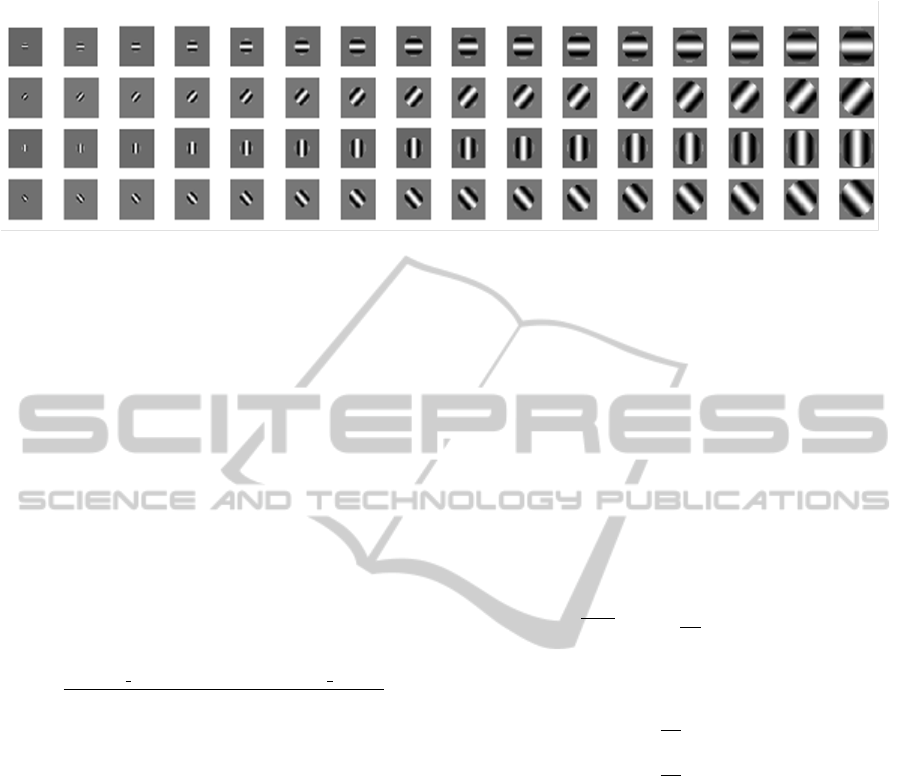
Figure 1: 64 Gabor filters (16 scales in steps of two pixels [7 × 7 to 37 × 37] × 4 orientations [0
◦
, 45
◦
, 90
◦
, 135
◦
]).
When α equals to 1, the reconstructed image is equiv-
alent to the equalized image. When α is chosen be-
tween ]1 2], then the singular values greater than unity
will be magnified. Thus, the combination between the
reconstructed image and the equalized image will be a
fruitful step to making the model more robust against
illumination and expression variations.
Interestingly, when the singular values are scaled in
the exponent, a non-linearity is introduced. Therefore
for a specific database (Caltech101 for example),
scaling down the magnification factor α may be
helpful.
Step 4 – Combined Image: The combined image
is produced by simply combining the reconstructed
image and the equalized image as shown in Figure
2, using a combination parameter c which varies
between 0 and 1.
I
Comb
=
Adapted Image + (c ∗ Reconstructed Image)
1 + c
(6)
By applying this approximation, the computations in
this layer become faster as shown in Figure 5 since
only the significant information are used for recogni-
tion. In addition, the approximation can significantly
improve the model’s accuracy. It can be explained by
the fact that when the model uses a challenge database
such as Calech101 or Caltech256 in which there are
a lot of unimportant information such as illumination
and expression variations, it will be interesting to ex-
ploit only the most important features in the images in
order to make the recognition easier and more robust
where the accuracy is increased by 10% using SVM
while by more than 13% when using NN classifier.
There are no related works yet that approximate the
S1 layer.
3.2 Combined Image-based HMAX
using Separable Gabor Filters
In this approximation, all the combined images of the
previous approximation are convolved with 64 Gabor
filters in a separable manner (G(x, y) = f (x)g(y)), in-
stead of just performing the 2-D convolution. In this
case, the Gabor features are computed using two 1-
D convolutions corresponding to convolution by f (x)
in the x-direction and g(y) in the y-direction. Based
on the definition of separable 2-D filters, the Gabor
filters are parallel to the image axes (θ = kπ/2). In
order to be applied to an image along diagonal direc-
tions, they have been extended to further work with
θ = kπ/4. The main issue of these techniques is that
they will not work with any other desired direction.
To handle this problem, eq. (1) can be rewritten us-
ing the isotropic version (γ = 1, circular) in the com-
plex domain (Chikkerur and Poggio, 2011). In this
case, u
2
+ v
2
= (xcosθ +ysinθ)
2
+ (−xsinθ +ycosθ)
2
= x
2
+ y
2
.
G(x,y)=e
−
x
2
+y
2
2σ
2
×cos
2π
λ
(x cos(θ)+y sin(θ)
= Re( f (x)g(y))
where
f (x) = e
−
x
2
2σ
2
× e
ix cos(θ)
,
g(y) = e
−
y
2
2σ
2
× e
iysin(θ)
.
Finally, the convolution using this approximation
can therefore be expressed as:
I
Comb
∗ G(x,y) = I
Comb
(x,y) ∗ f (x) ∗ g(y) (7)
By exploiting the separability of Gabor filters and
convolving them with the original image, the com-
putational complexity is reduced from O(N
2
M
2
) to
O(tN
2
M) where t=8 due to complex valued arith-
metic. But since in this approximation, the separable
Gabor filters are convolved with the combined image
I
Comb
, the complexity is being more reduced since
only the significant information are used for recog-
nition. The accuracy is not increased by more than
10.5% for SVM (between 10.4% and 10.5%) while is
increased by more than 14% for the NN classifier.
EfficientImplementationofaRecognitionSystemusingtheCortexVentralStreamModel
141
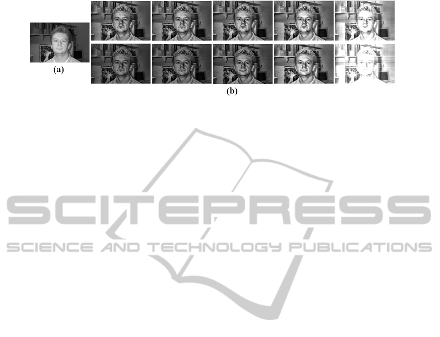
Figure 2: (a) The original image and (b) Combined images using α = 0.25, 0.5, 0.75, 1 and 1.25, respectively. c is equal to
0.25 and 0.75 on the top and bottom, respectively.
4 C1 LAYER APPROXIMATIONS
Concerning the C1 layer, a pooling between the S1 re-
sponses over scales within each band is performed by
simply taking the maximum response between them.
By testing what can be the result of the minimum
pooling that has not been exploited at this layer, it was
noticed that all the minimum scales values are very
close to their corresponding maximum ones. Some
of them are equal, otherwise the most of minimum
scales values are not smaller more than 6 or 7%. As
such, it will be important to further consider some of
the minimum scales values when taking the maximum
pooling. In other words, some of the minimum scales
values can be exploited in addition to the maximum
ones in order to increase the model’s accuracy. But
the remaining question to be solved is ”How to take
advantage of minimum and maximum scales values
at the same time”. So that under a specific conditions,
some of the minimum scales values can be embedded
into their corresponding maximum ones. The easiest
way to achieve that is to apply the embedding in the
additive domain. A general scheme of this approxi-
mation is shown in Figure 3. In this figure, two S1
image responses I
1
and I
2
of the same orientation at
the first band (band1) are considered and which are
belong to the filter scale 7 and 9, respectively. The cir-
cles shown within the images correspond to their pix-
els. In step 1, the maximum pooling (max function)
is performed between I
1
and I
2
. The pixels of the re-
sulting image correspond to the maximum scales val-
ues (shown with blue circles). In step 2, the mini-
mum pooling (min function) is performed between I
1
and I
2
. The pixels of the resulting image correspond
to the minimum scales values (shown with violet cir-
cles) that are then embedded into their corresponding
maximum ones in the additive domain under specific
conditions as shown in step 3. In other words, each
minimum scale value is added into the maximum one
that has the same (x, y) coordinates. w is the weight
of the embedding.
Embedding in the Additive Domain: This kind of
embedding is very straightforward to implement since
the minimum scales values (after applying the mini-
mum pooling over scales within each band) can be di-
rectly embedded into their corresponding maximum
values by simply using the addition operator.
Generally, the embedding process at a particular
pixel coordinate (x, y) in the additive domain can be
expressed as:
I
Embed
(x,y) = max
scale
(x,y) + w ∗ min
scale
(x,y), (8)
where I
Embed
(x,y) represents the final result after the
embedding process, max
scale
is the maximum scale
value, min
scale
is the minimum scale value, and w ∈
[0, 1] represents the weight of the embedding.
Two different conditions are considered to embed
the minimum scales values into their corresponding
maximum ones:
Condition 1: At each band, after computing the
maximum pooling over scales of the same orientation,
the minimum pooling is also performed and then all
the minimum scales values are embedded into their
corresponding maximum ones. In this case, w is set
to 1.
Condition 2: Each minimum scale value is embed-
ded if and only if its corresponding maximum value
belongs to the interval [0% 5%[. The values within
the interval specifies how much a maximum scale
value is greater than its corresponding minimum one.
In fact, the interval [0% 5%[ is divided into two
groups: [0% 2%[ and [2% 5%[, and two distinct sub-
conditions are thus considered:
• Sub-condition 1: The embedding is performed by
setting w to 1 for [0% 2%[ and 0.5 for [2% 5%[.
• Sub-condition 2: The embedding is performed by
setting w to 0.5 for [0% 2%[ and 0.1 for [2% 5%[.
The accuracy is not increased by more than 1% in
all conditions when SVM is used, while the opposite
for NN classifier. However, the computational com-
plexity at this layer is slightly increased due to the
embedding process.
VISAPP2015-InternationalConferenceonComputerVisionTheoryandApplications
142
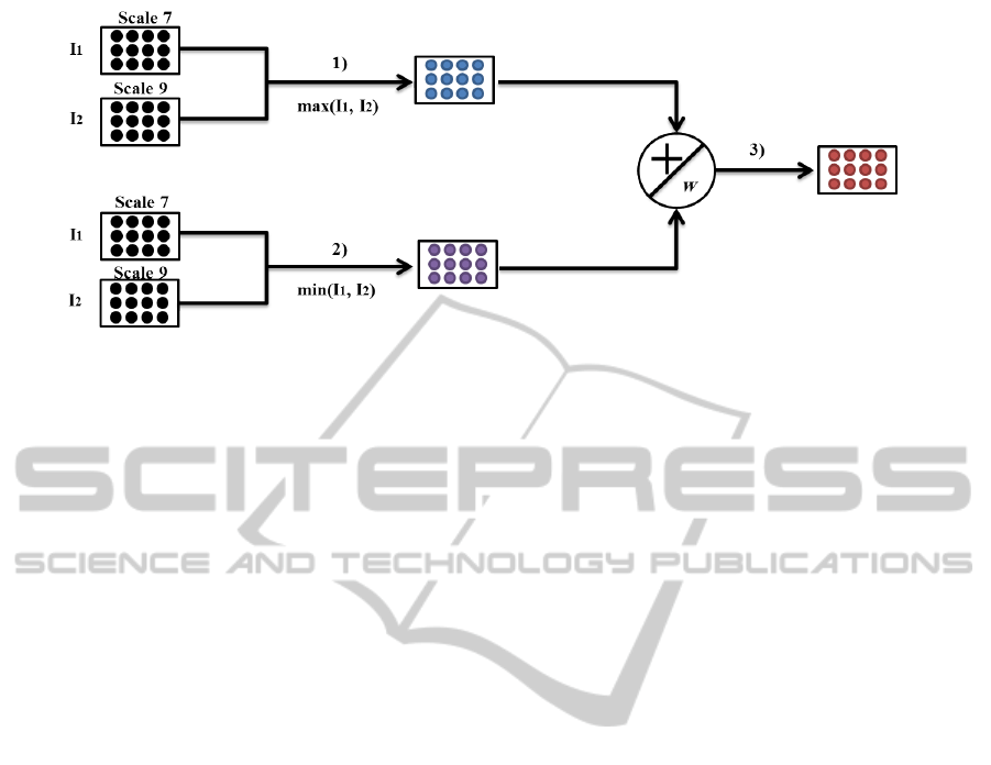
Figure 3: Scheme example of the C1 approximation.
5 S2 LAYER APPROXIMATIONS
At the S2 layer, the focus is to enhance the manner
by which all the prototypes are selected during the
feature learning stage. In the original model, P proto-
types are randomly selected from the training images
at the C1 layer. If more than P prototypes are used, the
model’s accuracy will increase at the expense of addi-
tional computational complexity. That is why our mo-
tivation is to learn the same number of prototypes P
but in an efficient way in order to decrease the model’s
false classification rate while keeping the same com-
putational complexity.
In order to achieve this, clustering is exploited,
which is considered one of the most important re-
search areas in the field of data mining. It aims to di-
vide the data into groups, (clusters) in such a way that
data of the same group are similar and those in other
groups are dissimilar. Clustering is considered useful
to obtain interesting patterns and structures. That is
why, one of the existing clustering algorithms, more
specifically the Partitioning Around Medoid (PAM)
clustering algorithm (Kumar and Wasan, 2011) has
been exploited in this approximation to generate the
prototypes.
Furthermore, one of the important issues to con-
sider, is the redundancy of some prototypes especially
those selected from the homogeneous areas of the
image (prototypes’ pixels are being equal to zero).
That is why, our contribution also aims to generate a
non-redundant P prototypes and force the model not
to generate any unimportant prototype. Accordingly,
each of the selected prototypes will be important and
aims to increase the model’s accuracy.
PAM is characterized by its robustness to the pres-
ence of noise and outliers. Its complexity is defined
by O(i(b − q)
2
) where i is the number of iterations,
q is the number of clusters, and b represents the total
number of objects in the data set.
To generate 2000 prototypes in a more efficient
way and use them in our model instead of the tradi-
tional ones, the PAM algorithm is performed and it
consists of 6 different steps:
Step 1 – 5 medoids of 4 × 4 pixels at four orientations
of each training category (total of 30 images) from
the total 102 categories are randomly initialized.
Step 2 – For each category, the Frobenius distance
between each of the C1 response of each image
with all the selected medoids is then computed in or-
der to associate each data image to the closest medoid.
Step 3 – For a random cluster, a non-medoid image
patch is randomly selected in order to be swaped
with the original medoid of the cluser in which the
non-medoid is selected.
Step 4 – steps 2 and 3 are repeated until the total cost
of swapping becomes greater than zero. The total cost
of swapping can be defined as follows:
Cost
swapping
= Current Total Cost − Past Total Cost
Step 5 –All the previous steps are also performed for
all the other remaining three sizes of the medoids (8
× 8, 12 ×12 and 16×16) in order to have a total of
20 medoids in each category.
Step 6 –Finally, a total of 2040 medoids are being
selected to be used as prototypes. 10 prototypes are
dropped from each size in order to end up with only
2000 prototypes.
This algorithm is complex since there are six steps
to perform in order to generate the prototypes. But in
fact, the run of the HMAX model relies on two parts.
The first part is responsible to generate and reserve all
the necessary prototypes by only running the first two
layers S1 and C1. The second part consists of running
the whole model and use the prototypes that have been
generated and reserved for the S2 layer. Interestingly,
EfficientImplementationofaRecognitionSystemusingtheCortexVentralStreamModel
143
the complexity of the model depends only on the sec-
ond part, which means that the large complexity of
our algorithm does not affect the computational com-
plexity of the model, more precisely, of the S2 layer.
That is why, the computational complexity at the S2
layer of our model remains O
PN
2
M
2
, where P is
the number of prototypes.
By applying this approximation, the accuracy of the
model incerases by 0.68% approximately using the
SVM classifier.
6 EXPERIMENTAL RESULTS
The proposed optimizations at the S1, C1 and S2 lay-
ers were implemented using MATLAB in order to
evaluate their accuracy and computational complexity
using experimental simulations. The S1, C1 and S2
approximations were evaluated using the Caltech101
database, which contains a total of 9,145 images split
between 101 distinct object categories in addition to
a background category. All the results of our approx-
imations were the average of 3 independent runs. For
each run, the following steps were performed:
1. A set of 30 images are randomly chosen from each
category for training, while all the remaining im-
ages are used for testing. All the images are nor-
malized to 140 pixels in height and the width is
rescaled accordingly so that the image aspect ra-
tio is preserved.
2. C1 sub-sampling ranges do not overlap in scales.
3. The prototypes are learned at random scales and
positions. They are extracted from all the eight
bands.
4. C2 vectors are built using the training set.
5. Training applied using both SVM and Nearest-
Neighbor classifiers.
6. C2 vectors for the test set are built, and then the
test images are classified.
6.1 Performance of SVM and NN
The performance of both SVM and NN are performed
on the face category extracted from the caltech101
database and which contains 435 face images. The
images were rescaled to 160 × 160 pixels, the C1
sub-sampling ranges overlap in scale (C1Overlap =
2) and the prototypes are chosen only from Bands 1
and 2. The classifiers were trained with n = 50, 100,
150, 200, 250, 300, 350 and 400 positive examples
and 50 negative examples from the background class,
while they are tested with all the remaining positive
examples and 50 examples from the negative set as
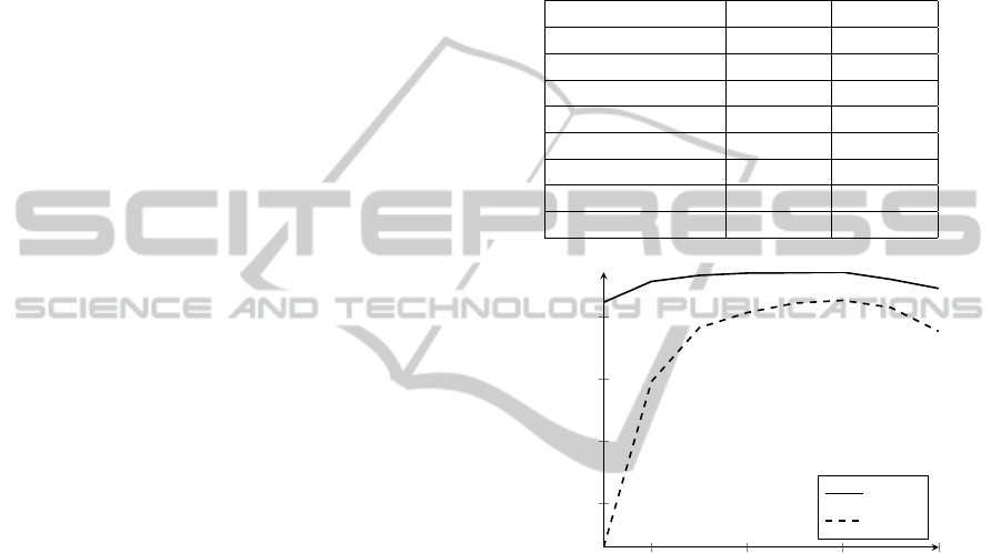
shown in Table 1 and Figure 4. 1000 prototypes (250
patches) × (4 sizes) are used in the S2 layer.
The results show that the accuracy decreases when
the number of training becomes greater than 300.
This is expected because the data becomes unbal-
anced.
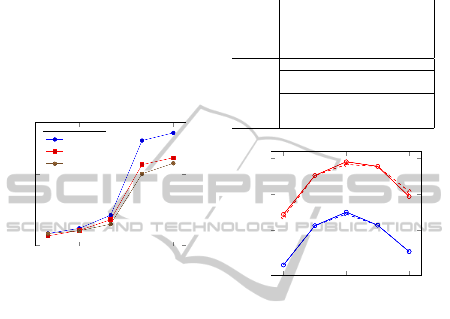
Table 1: Simulation results for SVM and NN on face cate-
gory.
Positive training SVM NN
50 92.325% 52.903%
100 95.678% 79.578%
150 96.656% 88.240%
200 97.018% 90.658%
250 97.075% 92.181%
300 97.165% 92.634%
350 96.019% 91.480%
400 94.558% 87.649%
100 200 300 400
60
70
80
90
Number o f positive training
Correct classi f ication rate (%)
SVM
NN
Figure 4: SVM and NN accuracies on face category.
6.2 Evaluations at the S1 Layer
At this layer, the computational complexity and cor-
rect classification rates (accuracies) for each of the
proposed approximations (Approx) are compared to
the baseline model.
• Approx1: Combined Image-based HMAX using
2-D Gabor filters.
• Approx2: Combined Image-based HMAX using
separable Gabor filters.
In order to compute the speed of the approximations
at this layer, the total time complexity of the S1 layer
is measured on a specific face image from the face
category. All the evaluations were done on a core i7
2.4 GHZ machine. The simulations were repeated five
times. Figure 5 illustrates an average of the results. It
shows that both Approx1 and Approx2 are faster than
VISAPP2015-InternationalConferenceonComputerVisionTheoryandApplications
144
the baseline (blue curve) for all the tested image sizes.
It has been noticed that for an image of size between
100x100 and 160x160, Approx1 is always faster than
Approx2. For example, Approx1 is faster than Ap-
prox2 by 3.23% for an image of size 100x100. For
other image sizes greater than or equal to 160x160,
Approx2 always shows lower timing than Approx1.
For example, for an image of size 160x160, Approx1
is faster than the baseline by 2.95% while by 3.42%
for Approx2. For an image of size 256x256, Approx1
is faster than the baseline by 6.29% while by 12.56%
for Approx2.
100x100
160x160
256x256
512x512
640x480
0
0.5
1
1.5
Time (s)
Baseline
Approx1
Approx2
Figure 5: Timing comparison (in s).
In order to assess the correct classification rates,
both SVM and NN classifiers were used. The average
accuracies of Approx1 under different values of α and
c are shown in Table 2. From all the following exper-
iments, 2000 prototypes (500patches) × (4 sizes) are
used and all the images were rescaled to 140 in height.
Recall that C1 sub-sampling ranges do not overlap in
scales and the prototypes are extracted from all the
eight bands. The performance of the original model
reaches 39% and 21.2% when using 30 training exam-
ples per class averaged over 3 repetitions under SVM
and NN, respectively. Table 2 proves our significant
contribution at the S1 layer especially for α = 0.75 and
c = 0.25 where the accuracy is increased by 10.02%
and 13.811% using SVM and NN, respectively.
Figure 6 illustrates the results shown in Table 2.
It shows 4 different curves. The red and blue solid
curves represent the accuracy values for c = 0.25 un-
der SVM and NN, respectively. While the red and
blue dashed curves are for c = 0.75 under SVM and
NN, respectively.
Finally, the separability of Gabor filters is ex-
ploited and applied to the combined image with α =
0.75 and c = 0.25. Approx2 shows an accuracy equal
to 49.471% and 35.372% for SVM and NN, respec-
tively.
Table 2: Classification accuracies of Approx1 approxima-
tion.
Approx1 Classifier c = 0.25 c = 0.75
α = 0.25 SVM 34.3652% 33.5927%
NN 20.284% 20.283
α = 0.5 SVM 45.201% 45.158%
NN 31.23% 31.231
α = 0.75 SVM 49.02% 48.269%
NN 35.011% 34.455%
α = 1 SVM 47.739% 47.739%
NN 31.362% 31.362%
α = 1.25 SVM 39.3531% 40.743
NN 23.998% 24.08%
0.25 0.5 0.75 1 1.25
20
30
40
50
α
accuracy (%)
Figure 6: Approx1 accuracies under different values of α
and c.
6.3 Evaluations at the C1 Layer
Figure 7 shows the average accuracies of the SVM
(blue x points) and NN (red x points) on several
C1 optimization options (Opt). The accuracy of the
model is increased a little bit when three cases of
the additive method are applied. For example, using
SVM, the accuracy is increased by 0.577%, 0.607%,
0.843% on Opt1, Opt2 and Opt3, respectively. On
the other hand, the increase is 0.846%, 1.88%, 1.85%
using NN.
• Opt1: Embedding all pixels (α = 1).
• Opt2: [0%,2%[, (α = 0.5); [2%,5%[, (α = 0.1)
• Opt3: [0%,2%[, (α = 1); [2%,5%[, (α = 0.5)
6.4 Evaluations at the S2 Layer
Table 3 shows the average accuracy of the SVM clas-
sifier based on the S2 approximation.
This approximation has a big advantage on
the model since the selected prototypes are non-
redundant and generated in more intelligent way.
EfficientImplementationofaRecognitionSystemusingtheCortexVentralStreamModel
145
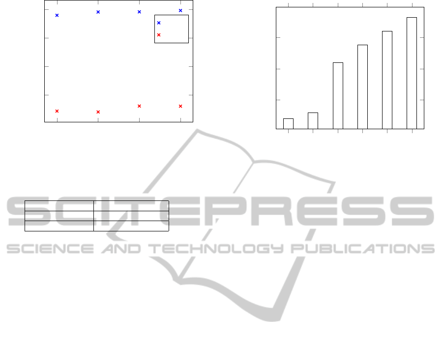
Baseline
Opt1
Opt2
Opt3
25
30
35
40
Accuracy (%)
SVM
NN
Figure 7: Average accuracies of C1 approximations.
Table 3: Accuracy of S2 approximation.
Approximation SVM
Baseline 39%
PAM 39.68% (+0.68%)
Therefore, each prototype serves to slightly increase
the accuracy. The accuracy of the model is increased
approximately by 0.68%.
6.5 Combined Classification Accuracies
Figure 8 shows the average accuracies of SVM on
the combination of the approximations ”Approx2” +
”Opt3” + ”PAM”. Our model shows an accuracy
equal to 51% when using only 2000 prototypes while
it shows 53.8% when using higher number of pro-
toypes (4080) as used by Serre et al. (2005b), Mutch
and Lowe (2006), Holub and Welling (2005), Grau-
man and Darrell (2005).
7 DISCUSSION AND FUTURE
WORK
In this study, the complexity of all the five different
layers of the original model of object recognition in
the visual cortex, HMAX, is presented. Different ap-
proximations were added to the first three layers S1,
C1 and S2.
The results showed that removing all unimportant in-
formation such as illumination, expression variations
and occlusions, to be a fruitful approach to improving
performance. The idea behind separability of Gabor
filters has been also exploited in order to be applied
on the combined images generated after keeping only
the important features for recognition. The change
of the main concept at the C1 layer is further applied
Serre et al. (2005b)
Holub and Welling (2005)
Our model
Our model’
Mutch and Lowe (2006)
Grauman and Darrell (2005)
45
50
55
42
43
51
53.8
56
58.2
Accuracy (%)
Figure 8: The accuracies of the final models.
by exploiting the advantage of some of the minimum
scales values and using them to be embedded into the
extracted maximum scales values. The accuracy was
slightly increased when the embedding process has
been applied using the additive method. Our model
serves also to always use an intelligent version of se-
lected prototypes at the S2 layer in order to remove
all the possibilities of having an unimportant proto-
type aiming to decrease the model’s accuracy.
As for future enhancements, a likely first step
would be to attempt to extend our work to the HMAX
model in color mode. In addition, several new ap-
proximations will be applied and tested on more chal-
lenging databases.
REFERENCES
Amayeh, G., Tavakkoli, A., and Bebis, G. (2009). Accurate
and efficient computation of gabor features in real-
time applications. In proceeding of the 5th Interna-
tional Symposium on Advances in Visual Computing:
Part I, volume 5875 of Lecture Notes in Computer Sci-
ence, pp. 243-252.
Bermudez-Contreras, E., Buxton, H., and Spier, E. (2008).
Attention can improve a simple model for object
recognition. In Image and Vision Computing, vol. 26,
pp. 776-787.
Cadieu, C., Kouh, M., Riesenhuber, M., and Poggio, T.
(2005). Shape representation in v4: Investigating
VISAPP2015-InternationalConferenceonComputerVisionTheoryandApplications
146

position-specific tuning for boundary conformation
with the standard model of object recognition. In Jour-
nal of vision, Vol. 5, no. 8.
Chikkerur, S. and Poggio, T. (2011). Approximations in
the hmax model. In MIT-CSAIL-TR-2011-021, CBCL-
298, 12p.
Grauman, K. and Darrell, T. (2005). The pyramid match
kernel: Discriminative classification with sets of im-
age features. In Proceedings of the IEEE International
Conference on Computer Vision (ICCV), pp. 1458 -
1465, vol. 2.
Holub, A. and Welling, M. (2005). Exploiting unlabelled
data for hybrid object classification. In Advances in
Neural Information Processing Systems (NIPS 2005)
Workshop in Inter-Class Transfer.
Kumar, P. and Wasan, S. K. (2011). Comparative study
of k-means, pam and rough k-means algorithms using
cancer datasets. In proceedings of CSIT: 2009 Inter-
national Symposium on Computing, Communication,
and Control (ISCCC Singapore, 2011, pp. 136–140.
Mutch, J. and Lowe, D. G. (2006). Multiclass object recog-
nition with sparse, localized features. In IEEE Con-
ference on Computer Vision and Pattern Recognition
(CVPR), vol.1, pp. 11-18.
Serre, T., Kouh, M., Cadieu, C., Knoblich, U., Kreiman,
G., and Poggio, T. (2005a). A theory of object
recognition: computations and circuits in the feedfor-
ward path of the ventral stream in primate visual cor-
tex. In CBCL Paper #259/AI Memo #2005-036, Mas-
sachusetts Institute of Technology, Cambridge, MA.
Serre, T., Kreiman, G., Kouh, M., Cadieu, C., Knoblich,
U., and Poggio, T. (2007a). A quantitative theory of
immediate visual recognition. In Progress in Brain
Research, Computational Neuroscience: Theoretical
Insights into Brain Function, vol. 165, pp. 33-56.
Serre, T. and Riesenhuber, M. (2004). Realistic model-
ing of simple and complex cell tuning in the hmax
model, and implications for invariant object recog-
nition in cortex. In Massachusetts Institute of Tech-
nology, Cambridge, MA. CBCL, Paper 239/Al Memo
2004-017.
Serre, T., Wolf, L., Bileschi, S., Riesenhuber, M., and
Poggio, T. (2007b). Robust object recognition with
cortex-like mechanisms. In IEEE Conference on Pat-
tern Analysis and Machine Intelligence, vol.29, pp.
411-426.
Serre, T., Wolf, L., and Poggio, T. (2005b). Object recogni-
tion with features inspired by visual cortex. In IEEE
Conference on Computer Vision and Pattern Recogni-
tion (CVPR’05), pp. 994-1000.
Sharif, M., Anis, S., Raza, M., and Mohsin, S. (2012). En-
hanced svd based face recognition. In Journal of Ap-
plied Computer Science & Mathematics, no. 12, p.49.
EfficientImplementationofaRecognitionSystemusingtheCortexVentralStreamModel
147
