Local Changes in Marching Cubes to Generate Less Degenerated

Triangles

Thiago F. Leal

1,2

, Aruquia B. M. Peixoto

, Cassia I. G. Silva

1,4

Marcelo de A. Dreux

and Carlos A. de Moura

Department of Mathematics, Rio de Janeiro Federal Institute, IFRJ, Paracambi, Rio de Janeiro, Brazil

Mechanical Engineering Doctorate Program, Rio de Janeiro State University, UERJ, Rio de Janeiro, Brazil

Department of Basic Disciplines, CEFET/RJ, Nova Iguaçu, Rio de Janeiro, Brazil

Computer Science Doctorate Program, Fluminense Federal University, UFF, Niteroi, Rio de Janeiro, Brazil

Mechanical Engineering Department, Rio de Janeiro Pontifical Catholic University, PUC-Rio, Rio de Janeiro, Brazil

Mathematics and Statistics Institute, Rio de Janeiro State University, UERJ, Rio de Janeiro, Brazil

Keywords: Implicit Surface, Marching Cubes, Computational Geometry.

Abstract: The Marching Cubes algorithm is widely used to generate surfaces from implicit functions. It builds a mesh

of triangles but many degenerated ones happen to appear among them, which can make the mesh thus built

unfit for many applications, like the Finite Element Method. To overcome this undesired behavior our work

proposes changes on the triangle generation that are automatically generated by Marching Cubes inside each

voxel. We first generate the polygon border inside each voxel that intersects the surface. Each polygon is

tested so as to guarantee the need to insert a new vertex inside itself, the triangles being then generated

according to each polygon properties in order to guarantee the best ratio between their sides and angles. The

resulting triangles inside each voxel exhibit the best possible ratio between their dimensions, thus leading to

a better mesh.

1 INTRODUCTION

Implicit functions are widely used to modeling

surfaces. They arise in the form of an algebraic

function or as a sampling in a grid, like functional

magnetic resonance imaging (FMRI), in medical

images.

In this work data remain in the space R

and the

implicit surface is defined as an isovalue set for the

implicit function. To define the isovalue as zero

means that all points for which f(x,y,z)=0 belong to

the surface. We will make a sampling of these points

in order to build a mesh that approximates the

surface thus defined.

There are many methods to generate an implicit

surface from an implicit function, like Marching

Cubes (Lorensen and Cline, 1987), Surface Nets

(Gibson, 1998), Extended Marching Cubes (Kobbelt

2001), Dual Marching Cubes (Nielson, 2004) and

Dual Contouring (Ju et al., 2002).

These methods start with a sampling of the the

implicit function values on a grid, which can be

either a uniform or an adaptive grid. Given that

sampling, every voxel from this grid is traversed to

find the voxels that intersect the surface, and one or

more vertex of the mesh are positioned in these

voxels, in order to be connected and generate the

mesh.

There are many different approaches to analyze a

mesh, but the most relevant are: topology, geometry

or quality of the mesh. Some works deal with the

topological characteristics of a surface in its

generation and/or simplification (Peixoto and

Moura, 2014), (Zomorodian, 2005), (Schaefer,

2007) and (Nielson and Hamann, 1991). If we look

towards geometrical characteristics, like curvature or

geodesics, some interesting works are (Martinez,

2005), (Velho et al., 2002) and (Wenger, 2005).

In this work we deal with the quality of

polygons, namely triangles, that generate an

unstructured mesh. The quality of the triangles in

this mesh is essential to many applications in

Engineering, like Finite Element Methods. Some

works deal with this characteristic (Dietrich 2009)

and (Gibson, 1998).

We propose a change in the Marching Cubes

143

F. Leal T., B. M. Peixoto A., I. G. Silva C., de A. Dreux M. and A. de Moura C..

Local Changes in Marching Cubes to Generate Less Degenerated Triangles.

DOI: 10.5220/0005309201430149

In Proceedings of the 10th International Conference on Computer Graphics Theory and Applications (GRAPP-2015), pages 143-149

ISBN: 978-989-758-087-1

 2015 SCITEPRESS (Science and Technology Publications, Lda.)

algorithm in order to generate a mesh of triangles

with better ratio between their sides and angles.

2 MARCHING CUBES AND

THEIR MODIFICATIONS

Marching Cubes (Lorensen and Cline, 1987) is an

algorithm that generates a tridimensional

representation of the border of a volume. The

surface is polygonized, with the values of an implicit

function being used to positioning the vertex points

of the mesh that generates the triangles of the

approximating surface.

Its first application was carried on for medical

images, where a series of bi-dimensional images

slices makes it possible to computationally

reconstruct a model for the patient anatomy. This

turns much easier the generation and visualization of

medical images for traumas and broken bones.

Nowadays Marching Cubes is widely employed

in many other areas that need to generate a surface

from an implicit function, from animation to

different engineering applications.

2.1 Marching Cubes

Marching Cubes starts with a cube that contains the

surface. Each axis of this cube is subdivided, thus

generating a grid with new small cubes, the voxels.

Each voxel is transverse and if it intersects the

surface, the vertex of the mesh is generated, being

positioned in the border of each voxel. These

vertices are automatically connected to generate the

triangles inside this voxel. The algorithm moves to

the next voxel so as to generate the next triangles.

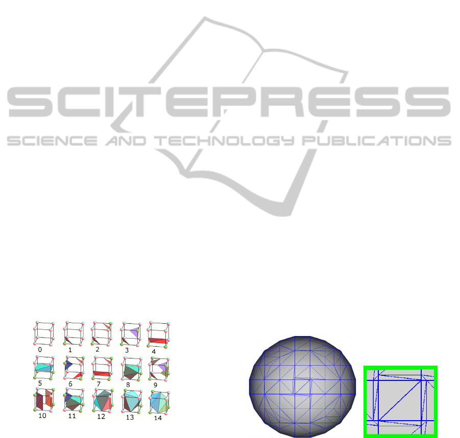
Figure 1: Marching Cubes: The original 15 configurations.

The original MC uses a table with 15 possible

configurations, except rotation, to decide how to

automatically generate the triangles, as shown in

figure 1.

2.2 Topological Ambiguities

After the original configurations presented in

Marching Cubes, some cases with topological

ambiguity arise. In these cases, we can have two

options to connect the vertex of the mesh inside a

voxel. These options can generate two completely

distinct topological configurations, e.g. one with a

connected surface and another one with two or more

disconnected surfaces.

Some techniques were created to deal with these

flaws (Lorensen and Cline, 1987), (Chernyaev,

1995). These works take the original 15

configurations and expand them to 33 final

configurations, without ambiguity of the resulting

surface topology.

Even with these new configurations, the structure

inside each voxel remains the same, with the

algorithm automatically generating the mesh

triangles. After the voxel traverse the whole grid, the

mesh is generated with all triangles, as shown in

figure 2, right.

2.3 Degenerated Triangles

The Marching Cubes algorithm can lead to some

difficulties, due to the limitation in the use of an

automated triangle generation. It is common to get

hold of degenerated triangles, by which it is meant

the existence of a very small edge or angle, as

compared to the two others. For numerical

applications, such triangles can lead to unstability,

so that the solution fails to be reached by the

numerical method.

Figure 2 shows a detail of a sphere polygonised

with the Marching Cubes algorithm. We can see

some degenerated triangles, mainly in the sphere

center.

Figure 2: Polygonization of a sphere, with the details of

triangles on the mesh center.

GRAPP2015-InternationalConferenceonComputerGraphicsTheoryandApplications

144

3 LOCAL CHANGE

The changes in Marching Cubes algorithm herein

proposed are performed only inside each voxel

during the polygonization. In short, in this work we

do not look at the neighbors of this voxel. That is the

reason why we call this change a “Local Change”.

In the cases where isolated triangles appear

inside a voxel, nothing is done with these triangles.

For example, figure 3 shows some cases where the

voxel generates isolated triangles. Only the

configurations 7 and 11 can have changes in the

triangles connections, because they have polygons

with four and five edges, respectively.

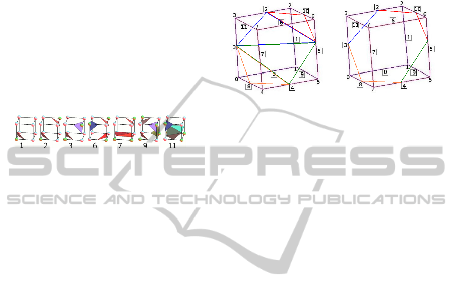
Figure 3: Some Marching Cubes configurations that

contain isolated triangles.

The algorithm proposed in this work is composed by

four steps:

 Generate the border of each polygon

 Separate the vertex with a bad angle

 Insert a new vertex, if necessary

 Connect the vertex.

3.1 Generate the Border of Each

Polygon

The first step is to change the Marching Cubes table.

The original table automatically generates the

triangles. For every possible configuration and

positioning, Marching Cubes choses a vector with

the voxel edges that intersect the surface. For each

of these edges the positioning of the vertex that

generates the triangles of the mesh is calculated.

Each sequence of the vector three elements

corresponds to a triangle.

In our algorithm, we change this vector with the

first entries being the isolated triangles, if they exist.

After this step, if there is a polygon with four or

more sides, a flag-2 is used to indicate that the next

entries are the border of this polygon, and not a

triangle.

Figure 4 shows, in the left, the triangles

automatically generated by Marching Cubes. This

case gives the vector {2, 10, 5, 3, 2, 5, 3, 5, 4, 3, 4,

8, -1, -1, -1, -1}, where we have four triangles

generated by the edges of the voxel (2, 10, 5), (3, 2,

5), (3, 5, 4) and (3, 4, 8). In the right, we have the

vector {-2, 2, 10, 5, 4, 8, 3, -1, -1, -1, -1, -1, -1, -1, -

1, -1}. Since we do not have isolated triangles, only

a polygon with five edges, then the vector starts with

the flag “-2”, to indicate that we have only the

border of a polygon, and we have the five edges of

the voxel that defines this polygon (2, 10, 5, 4, 8, 3).

Figure 4: Marching Cubes triangles and configurations. a)

The original Marching Cubes triangles {2, 10, 5, 3, 2, 5, 3,

5, 4, 3, 4, 8, -1, -1, -1, -1}, b) Modified Marching Cubes

table {-2, 2, 10, 5, 4, 8, 3, -1, -1, -1, -1, -1, -1, -1, -1, -1}.

3.2 Separate the Vertex with a Bad

Angle

This work deals with the local changes that are done

inside a single voxel. For this reason we fail to have

information about the neighbours of a voxel. If a

vertex of the polygon inside a voxel has a too small

angle, no information about their neighbours is

available to produce any change for this angle.

This case of too small angles will be treated in

another work, where we have access to the entire

mesh. To prevent that this small angle makes the

mesh still worst, we will not split it.

We create an edge connecting the two vertexes

that are connected to this vertex, thus getting a new

triangle. If in this case we cannot make a better

angle, at least we do not create triangles with worst

angles, and let this small angle be isolated so as to

be treated in a global change.

Figure 5 shows a polygon with a vertex, on the

top, with a small angle. At the left it shows the

triangles automatically generated by Marching

Cubes: three new triangles with worse angles. Our

algorithm is shown at the right, where we take the

small angle and connect their neighbours, creating

one triangle with a bad angle. With the local

changes, we cannot make this angle better, but we

do not create triangles with angles worse than the

ones of the polygon original border.

LocalChangesinMarchingCubestoGenerateLessDegeneratedTriangles

145

Figure 5: Polygon with a bad angle on his top. a)

Automatic triangulation due to Marching Cubes. b) Our

algorithm, that prevents to split the bad angle.

3.3 Insert a New Vertex

After each vertex with a bad angle is marked, to

prevent its splitting, we analyse the remaining

polygon to check up whether it is necessary to

position a new vertex inside it. This new vertex is

used to generate triangles with better angles, but

note: it is positioned only in four or more edge

polygons.

In the case of a four edge polygon, the ratio of

the bigger and the smaller edges are analysed, and if

they remain bellow a threshold, indicating that there

is a significant difference between these edges, then

a new vertex is positioned inside this polygon. For

all polygons with five or more edges, a new vertex is

inserted. This new vertex is placed closer to the

smaller one. It may be thought that an attraction

force pulls this new vertex closer to the smaller

edges.

Every vertex of the polygon is connected to two

edges. To every vertex we calculate the length of the

smallest edge (LSE), and we associate this

information to the edge. We make a sum of all the

lengths associated to these vertices (SLME).

With these information we create an attraction

factor √(1 + SLME/LSE) to every vertex. The final

position of the new vertex is the sum of every

position of the vertices of the polygon multiplied by

this attraction factor.

In this work, we only use the vertex that

generates the border to positioning the new vertex,

because it is a local change, where we do not have

access to the voxel neighbours. We do not position

the new vertex close to the surface, using the

implicit function, because we can generate structures

like pyramids inside a voxel, even in smooth

surfaces, what to applications in numerical methods

can generate unstable results.

With this positioning, this new edge is closer to

the smaller edges, generating new triangles with

better ration between their sides. Figure 6 shows two

possible positions for a new vertex inside a polygon.

At the left, the new vertex is positioned on the

polygon center, and at the right, the positioning of

the new vertex is closer to the smaller edge. In this

figure, we can see that the triangles generated at the

left show better quality between their sides and

angles.

Figure 6: Positioning a new vertex inside a polygon. a)

Positioning in the center. b) Positioning closer to the

smallest edge.

3.4 Connect the Vertex

There are two cases to connect the vertex of a

polygon: if there is a new inserted vertex inside the

polygon, or if there is only the original border

vertex.

If there is a new vertex inserted inside the

remaining polygon, then all polygon vertices are

connected to them, as shown in Figure 6.

When there is no vertex inside the polygon, we

choose the vertex with biggest angle. It will be

connected to the border vertex that is at a distance of

two edges, and that has a bigger angle. With this

procedure, the bigger angles are split, thus

generating triangles with better angles.

Figure 7 right shows an automatic triangulation

made by Marching Cubes, where a big angle on the

top left remains as a big angle in the triangle. In the

left, we split this angle, generating two triangles

with better angle in this vertex.

Figure 7: Generating triangles from the border of a

polygon. a) Automatic triangulation, due to Marching

Cubes. b) Our algorithm, that splits the bigger angle.

4 RESULTS

To analyse the results, we use a histogram to see the

GRAPP2015-InternationalConferenceonComputerGraphicsTheoryandApplications

146

angles distribution. The axis x corresponds to the

angles, where each interval has a size of five angles,

and the axis y shows the number of vertices that

have angles in this interval.

The algorithm presented in this work can

introduce one vertex inside some voxels. With this,

the total numbers of triangles, and vertices, can be

different for a surface polygonised with Marching

Cubes and with our algorithm.

In order to see the difference between the

meshes generated with Marching Cubes and our

algorithm, we draw the borders of the triangles in

the mesh. To have a better analysis of the

distribution of the angles, we show the histogram of

every surface. We analyse three surfaces: a sphere, a

hyperboloid and a grid with many holes.

4.1 Sphere

We start with a sphere that is polygonized using a

grid with ten subdivisions in each axis, generating

voxels. With this very coarse grid, we can see

the mesh with more details, with the triangles that

generate the mesh.

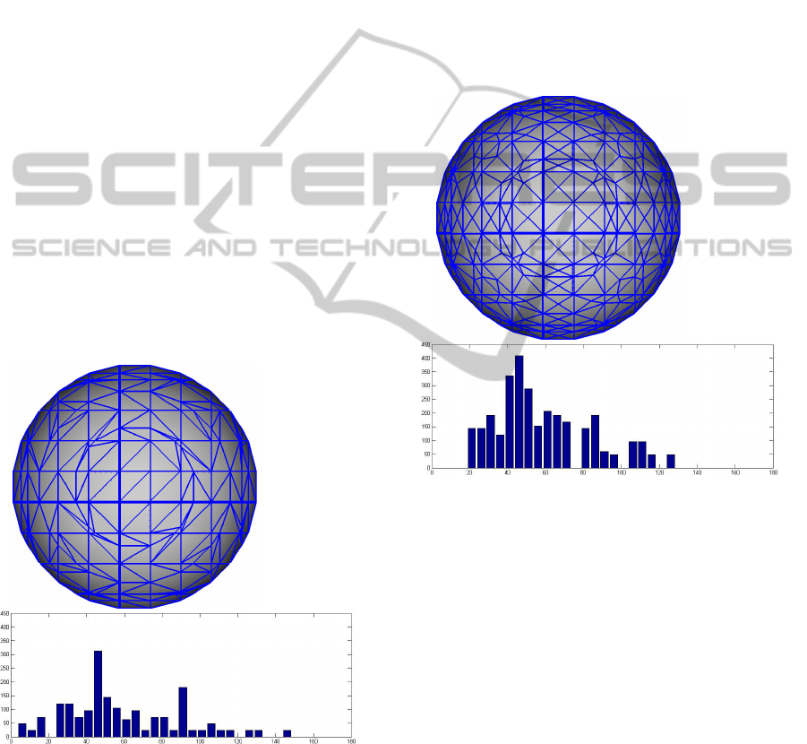
The figure 8 shows a polygonization done with

Marching Cubes. In this case we can see many

degenerated triangles around the sphere center.

Figure 8: Sphere polygonized with Marching Cubes, and

the histogram with the distribution of the angles. There are

524 triangles in this mesh.

On the histogram of this distribution we can see

a peak in the interval 45-50, and another smaller

peak in the interval 90-95. The remaining angles

show a distribution much more dispersed, like a

statistical uniform distribution. In this surface, there

is a significant number of vertices with angles

between 5 to 20 degrees, and the angles of the

triangles are in the interval 5 to 145 degrees.

Figure 9 shows the polygonization of the same

sphere, with the same grid, using the algorithm

presented in this work. We can see that the triangles

around the sphere center have better angles, and the

ratio between their sides are better too.

The histogram shows that the angles are more

concentrated around the interval 45-50, with less

dispersion, and the smallest angle starts with 20

degrees. In this case, the angles of the triangles are

in the interval 20 to 130 degrees.

Figure 9: Sphere polygonized with the algorithm presented

in this work, and the histogram with the distribution of the

angles. There are 852 triangles in this mesh.

4.2 Hyperboloid

The surfaces presented in this section, and in the

next, are polygonised with a less coarse grid, each

axis has forty subdivisions, generating 40

voxels.

This makes it easier to analyse the distribution of the

angles of the triangles, but a little more difficult to

see the triangles that generate the mesh.

The hyperboloid generated by Marching Cubes is

shown in figure 10. Even with a grid with many

subdivisions, that generates many triangles, we can

see that there are many triangles with small angles.

The histogram has a peak on the interval 50-55,

and there is a significant amount of angles in the

interval 0-5. The angles of the triangles are in the

interval 0 to 170 degrees, with a big dispersion.

LocalChangesinMarchingCubestoGenerateLessDegeneratedTriangles

147

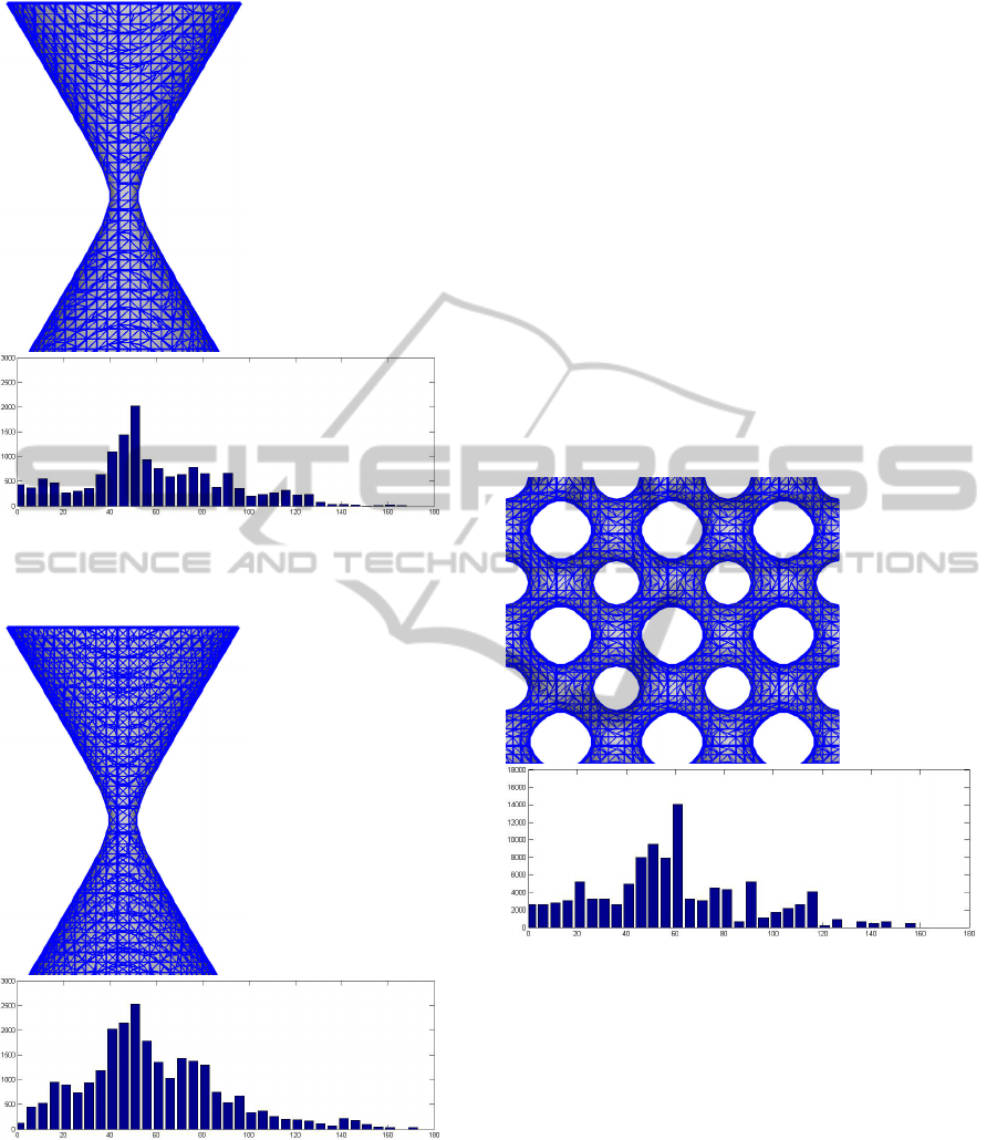
Figure 10: Hyperboloid polygonized with Marching

Cubes, and the histogram with the distribution of the

angles. There are 15308 triangles in this mesh.

Figure 11: Hyperboloid polygonized with the algorithm

presented in this work, and the histogram with the

distribution of the angles. There are 25179 triangles in this

mesh.

Figure 11 shows the polygonization of the

samehyperboloid, with the same grid, using the

algorithm presented in this work.

The mesh on the surface shows that the triangles

have better angles, and some new vertex was

introduced to generate this mesh.

The histogram shows that the angles are more

concentrated around the interval 50-55, with less

dispersion. The amount of angles in the interval 0-5

decrease, even with more triangles in this mesh.

4.3 The Grid

The Grid is a surface generated with cosines that is a

tube involving a grid, generating many holes.

Figures 12 and 13 show a front view of this surface.

In figure 12 we can see the surface polygonized

with Marching Cubes. We can see that there are

many triangles with small angles.

The histogram shows a peak in the interval 50-

55, a significant amount of angles in the interval 0-5,

and the angles are more dispersed.

Figure 12: The Grid polygonized with Marching Cubes,

and the histogram with the distribution of the angles.

There are 10457 triangles in this mesh.

Figure 13 shows the same Grid, but polygonized

with our algorithm. In this figure, there are less

triangles with small angles. The histogram shows a

peak in the interval 50-55, but in this case, the

angles are less dispersed, being concentrated around

this peak.

5 CONCLUSIONS AND FUTURE

WORKS

This work deals with the local changes in Marching

GRAPP2015-InternationalConferenceonComputerGraphicsTheoryandApplications

148

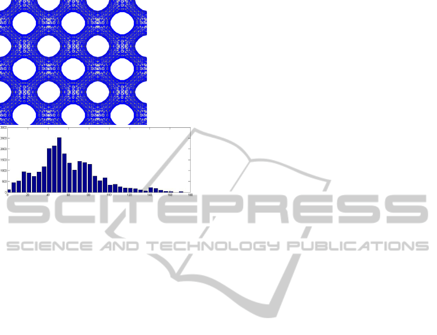
Figure 13: The Grid polygonized with the algorithm

presented in this work, and the histogram with the

distribution of the angles. There are 25077 triangles in this

mesh.

Cubes algorithm. These changes are performed only

inside a voxel, with no information about the

neighbours, this is the reason why these changes are

called local changes.

We can see, analyzing the triangles of the mesh

that are drawn on the surface, that the mesh resulting

from these changes has better triangles, with better

angles and better ratio between their sides.

The histograms of the surfaces polygonized with

Marching Cubes have some peaks, but the angles are

more dispersed, closer to a uniform distribution. All

histograms of the surfaces polygonized with the

algorithm presented in this work show an angles

concentration around the interval 40-60, and less

angles dispersion.

In future works we can use information from the

entire mesh, repositioning the vertex with small

angles, which are in the border of the polygon, thus

generating a mesh with better angles triangles.

Another approach is to deal not just with a surface,

but with an entire volume.

REFERENCES

Dietrich C. A., Scheidegger C., Comba J. L. D., Nedel

L.P., Silva C. T., 2009, Marching cubes without skinny

triangles, Computing In Science & Engineering, Vol.

11, No. 2. pp 82-87.

Chernyaev, E. V., 1995. Marching Cubes 33:

Construction of Topologically Correct Isosurfaces,

Technical Report CERN CN 95–17, CERN.

Gibson, S. F. F., 1998, Constrained Elastic Surface Nets:

Generating Smooth Surfaces from Binary Segmented

Data, Proceedings of the First International

Conference on Medical Image Computing and

Computer-Assisted Intervention, MICCAI, pp. 888-

898.

Ju, T., Losasso, F., Schaefer, S., Warren, J., 2002, Dual

Contouring of Hermite Data, Proceedings of the 29th

Annual Conference on Computer Graphics and

Interactive Techniques, SIGGRAPH 2002. Pp. 339-

346.

Kobbelt, L. P., Botsch, M., Schwanecke, U., Seidel, H-P.,

2001, Feature Sensitive Surface Extraction from

Volume Data, Proceedings of the 28th Annual

Conference on Computer Graphics and Interactive

Techniques, SIGGRAPH 2001. pp 57-66.

Lorensen, W. E., Cline, H. E., 1987. Marching cubes: A

high resolution 3D surface construction algorithm,

Proceedings of the 14th annual conference on

Computer graphics and interactive techniques, pp.163-

169.

Martinez, D., Velho, L., Carvalho, P. C., 2005, Computing

Geodesics on Triangular Meshes. Computers &

Graphics v. 29, n.5, p. 667-675.

Nielson, G. M., Hamann, B., 1991. The Asymptotic

Decider: Resolving the Ambiguity in Marching Cubes,

Proceedings of the 2

Conference on Visualization '91,

VIS 91, pp. 83-91, IEEE Computer Society Press.

Nielson, G. M., 2004, Dual Marching Cubes, Proceedings

of the Conference on Visualization 2004, VIS 2004.

Pp. 489-496.

Peixoto, A. B. M., Moura, C. de, 2014, Topology

Preserving Algorithms for Implicit Surfaces

Simplifying and Sewing, Proceedings of 14th

International Computational Science and Its

Applications – ICCSA. pp. 352-367.

Schaefer, S., Ju, T., Warren, J., 2007, Manifold Dual

Contouring, IEEE Transactions on Visualization and

Computer Graphics. Pp. 610-619.

Shewchuk, J. R., 2002, What Is a Good Linear Finite

Element? - Interpolation, Conditioning, Anisotropy,

and Quality Measures. In Proc. of the 11th

International Meshing Roundtable, p. 115-126.

Velho, L, Figueiredo, L. H., Gomes, J, 2002, Implicit

Objects in Computer Graphics, Springer.

Wenger, A., 2005, Isosurfaces: Geometry, Topology, and

Algorithms, Taylor & Francis.

Zomorodian, R., 2005, Topology for Computing,

Cambridge: Cambridge University Press.

LocalChangesinMarchingCubestoGenerateLessDegeneratedTriangles

149