Point Cloud Structural Parts Extraction based on Segmentation Energy

Minimization

Bruno Cafaro, Iman Azimi, Valsamis Ntouskos, Fiora Pirri and Manuel Ruiz

Department of Computer Science, “Sapienza” University of Rome, Via L. Ariosto, 25, Rome, Italy

Keywords:

Point Clouds, Level Set Methods, Minimal Surface Energy, Segmentation, Meshing.

Abstract:

In this work we consider 3D point sets, which in a typical setting represent unorganized point clouds. Segmen-

tation of these point sets requires ﬁrst to single out structural components of the unknown surface discretely

approximated by the point cloud. Structural components, in turn, are surface patches approximating unknown

parts of elementary geometric structures, such as planes, ellipsoids, spheres and so on. The approach used

is based on level set methods computing the moving front of the surface and tracing the interfaces between

different parts of it. Level set methods are widely recognized to be one of the most efﬁcient methods to seg-

ment both 2D images and 3D medical images. Level set methods for 3D segmentation have recently received

an increasing interest. We contribute by proposing a novel approach for raw point sets. Based on the motion

and distance functions of the level set we introduce four energy minimization models, which are used for

segmentation, by considering an equal number of distance functions speciﬁed by geometric features. Finally

we evaluate the proposed algorithm on point sets simulating unorganized point clouds.

1 INTRODUCTION

This work is focused on 3D point cloud analysis.

These are geometric data sets in which only the digi-

tized 3D points are usually available. Such low-level

data exhibits a huge gap with a high-level representa-

tion, which is necessary in many application areas as:

surface compression, shape classiﬁcation, hybrid ren-

dering, meshing or simpliﬁcation. We deﬁne simple

scene elements, to extract their structural parts, rely-

ing only on the raw point cloud. The proposed frame-

work is based on energy minimization using Level Set

and the construction of speciﬁc distance functions us-

ing local geometric features, such as normals, surface

variation and height of points. The novelty is due to

the contextually guided mesh construction, which ap-

proximates the minimal surface energy of the consid-

ered structural components. More precisely, the pro-

posed approach forms a mesh from a set of points

only if these points share common local geometric

features. Here we assume that structural parts of a

simple scene element can be characterized by com-

mon geometric features values. Iteratively repeating

the mesh construction for each structural part, seg-

mentation is obtained, as can be seen in Figure 1.

The level set based approach proves to be quite

general as it performs extremely well in surface en-

ergy minimization, despite it takes into account just

few parameters. We tested the proposed method

on point sets simulating unorganized point clouds

of scene elements, highlighting the composition of

structural parts, and adding typical points cloud noise

level. Extension of this segmentation framework to

more complex scene elements and very large point

clouds might require some further work, though we

expect that most of the approach can be elegantly gen-

eralized.

The paper is organized as follows: in Section 2

we review state of the art on 3D segmentation; in

Section 3 we introduce the level set framework for

surface reconstruction. In Section 4 we introduce the

voxel space and the proposed 3D segmentation meth-

ods. Section 5 explains the main implementation is-

sues and Section 6 illustrates the performed experi-

ments. Finally, in the conclusion we address how the

method could be used for object segmentation.

2 RELATED WORKS

Our approach is based on raw point cloud analysis,

and survey (Nguyen and Le, 13) summarizes recent

approaches for unorganized point cloud segmenta-

tion. The author propose to classify the segmentation

150

Cafaro B., Azimi I., Ntouskos V., Pirri F. and Ruiz M..

Point Cloud Structural Parts Extraction based on Segmentation Energy Minimization.

DOI: 10.5220/0005309301500157

In Proceedings of the 10th International Conference on Computer Graphics Theory and Applications (GRAPP-2015), pages 150-157

ISBN: 978-989-758-087-1

 2015 SCITEPRESS (Science and Technology Publications, Lda.)

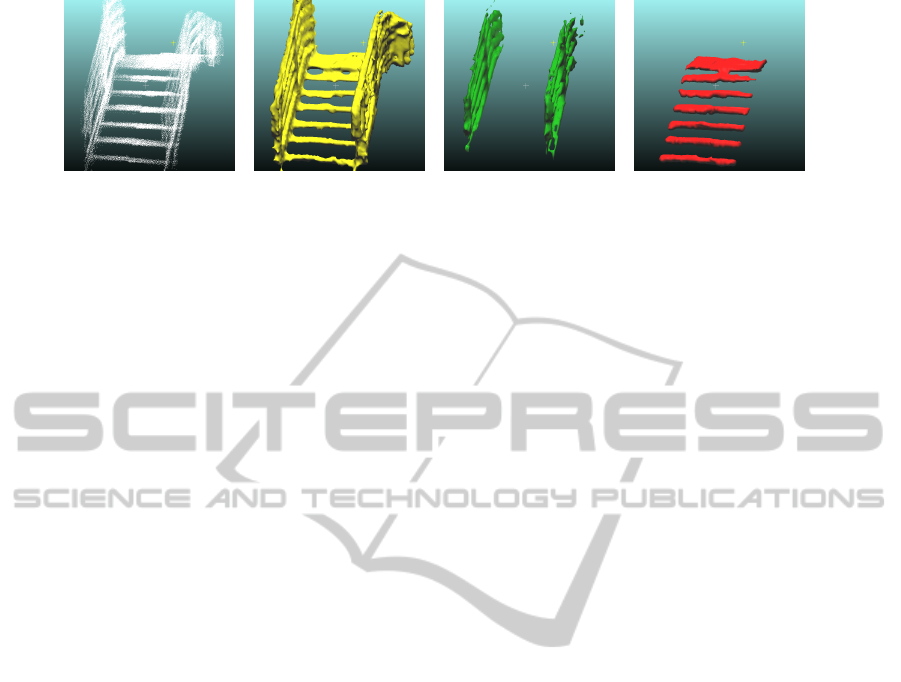
Figure 1: Results of model M

segmentation and meshing on unorganized 3D laser scan data.

methods in ﬁve main methods: edge based, attribute

based, graph based, region based, and model based.

Among the edge based methods, (Ioannou et al., 12)

propose to segment points adopting a difference of

normal (DoN) operator. In (Rusu, 09) the author pro-

poses an attribute based method exploiting euclidean

clustering, and plane ﬁtting, creating a queue for not

labeled points, which are further assigned to one of

the clusters according to features distance. Amid the

graph based methods, (Ma et al., 10) propose to par-

tition the point cloud data adopting a graph min-cut

procedure, where the graph is deﬁned according to

points similarity; then spectral clustering is used to

solve min-cut. In (Nurunnabi et al., 12) region grow-

ing exploits features such as color, normal vectors or

curvature. In (Golovinskiy and Funkhouser, 09) the

proposed graph-cut method computes an edge cost

between points, and between points and source, and

points and sink. Then a min-cut, max-ﬂow approach

is used to cut the created graph. In model based meth-

ods points are grouped using geometric primitives.

In (Kustra et al., 2014) the authors ﬁrst estimate

surface properties, then apply clustering in the Gauss

sphere to group points in patches. Those are classiﬁed

using a connectivity graph.

Other approaches develop on available mesh con-

nectivity, extracting information also from the edges

or the polygons of the mesh itself, for a review see

(Shamir, 08) and references therein. Also mesh seg-

mentation is grouped in ﬁve methods: region grow-

ing, hierarchical clustering, iterative clustering, spec-

tral analysis and implicit methods. In iterative clus-

tering the segmentation is formulated as a variational

problem, then a solution is iteratively searched for the

given number of clusters, see for example (Lloyd, 06).

In (Karni and Gotsman, 00) spectral clustering ex-

ploits the same principles for meshes and point sets,

but computing the Laplacian matrix for mesh ver-

tices. In (Schreiner et al., 04) a mesh is divided into

its parametrized surfaces of simplicial domains. Ob-

viously many of the approaches for raw point cloud

data share some common features with mesh based

approaches, and can be easily implemented on both

data structures, except for implicit methods.

The problem of most of these methods with re-

spect to the one proposed in this paper is the lack of a

clear mathematical framework that allows for a paral-

lel computation, essential for large point clouds. This

aspect is not true in Level Set based methods for med-

ical image analysis (see survey (Wirjadi, 07) and ref-

erences therein). Those methods can be applied when

a volumetric representation of the data is available,

and are based on implicit functions evolution, extend-

ing and reﬁning the Chan-Vese algorithm for 2D im-

ages on 3D images.

Other works share common features with our ap-

proach, but are based on completely different mathe-

matical framework. An example is (Schnabel et al.,

07), in which a RANSAC based algorithm is used

to detect clusters of 3D points which belongs to the

same geometrical shape: planes, spheres, cylinders,

cones and tori. This approach has been reﬁned and

extended to cope also with sharp edges in (Tran et al.,

14). In (Turner and Zakhor, 14) the authors develop

an approach based on the extrusion of the 2D map of

a storey, then adding soil and ceiling to obtain a wa-

tertight mesh of that storey.

The roots of the proposed approach can be found

in (Zhao et al., 98; Zhao et al., 01; Liang et al., 13),

in which the authors solve the problem of surface re-

construction. These methods are suited for watertight

reconstruction of an entire object. In (Liang et al., 13)

the inner product ﬁeld is used to compute a signed

distance function whose zero lies close to the sur-

face approximated by the input points. We extend this

method by forming a mesh only for the input points

which share common predetermined geometric fea-

ture values.

3 PRELIMINARIES AND THE

LEVEL SET METHODS

Level set methods are numerical techniques widely

adopted in computational physics, ﬂuid-dynamics,

computer vision, graphics, and many others ﬁelds, for

tracking interface evolution and shapes in many dif-

ferent kind of mediums. The great advantage over

PointCloudStructuralPartsExtractionbasedonSegmentationEnergyMinimization

151

other methods is the possibility to perform numerical

computations involving curves and surfaces on a ﬁxed

Cartesian grid, without having to parameterize these

objects, but using their implicit deﬁnition instead.

Notation: In the following we shall use boldface

letters, both lower and upper case, for vectors, matri-

ces and vector ﬁelds such as x, w,v, X. We denote

time with t, and use lower-case Greek letters for func-

tions: ρ is used in particular for the distance func-

tion and φ for the level set function. We make argu-

ments of a function explicit only when needed: we

may write φ(w,t), φ(t) or φ(w). We reserve upper

case Greek or Latin letters for sets, in particular the

point set is denoted S and the domain Ω. Points in Ω

are denoted w, and points in S by x, s or x

as we indi-

cate with the subscript i the i-th elements of a vector,

matrix or set. For the inner product we use both the ·

or nothing, and in this last case we make explicit the

transpose with the top > as superscript. The partial

derivative of a function ϕ with respect to parameter w

is indicated by ϕ

. Finally, we indicate by k·k the

Euclidean norm, by |·| the absolute value.

By structural component of a simple scene ele-

ment we intend that part of a point cloud approxi-

mating an unknown surface patch that could not be

split into simpler elements. Within a scene element

a structural component cannot be broken down into

other scene elements of different kinds. In turn, by a

simple scene element we intend any part of a complex

scene.

Let Ω be a domain in the 3D Euclidean space,

let w = (x,y, z)

∈ R

and φ : Ω ×R 7→ R, then the

boundary among two regions, within Ω, can be spec-

iﬁed according to an implicit representation: ∂Ω =

{w | φ(w) = 0}. The surface separating these two

regions is the zero level of the function φ(w), called

the level set function. When adopting a level set ap-

proach, one usually starts with an initial guess for

the level set function. Then the guessed function is

evolved considering an algorithmic time, up to con-

vergence to a minimum. This minimum is found

deﬁning another function governing the level set evo-

lution, which is usually a signed or unsigned distance

function. Typically the distance function from a point

w to a set S is deﬁned:

ρ(S,w) = min

∈S

(kw −x

k) (1)

Which implies that when S is the boundary ∂Ω, and

w ∈ ∂Ω, then ρ(∂Ω,w) = 0.

Adopting the Eulerian approach, which is the

same as observing the variation of the level set func-

tion φ(w) in a given location in space, different mod-

els for the evolution of φ(w) can be deﬁned. The level

set equation is deﬁned as:

(t) + v ·∇φ(t) = 0. (2)

Here v is the velocity which governs the level set evo-

lution.

3.1 Minimal Surface Energy Model

The level set function φ embeds the surface separating

two regions, during its evolution. If we consider the

samples collected from the surface of an object, such

as S = {x

,.. . ,x

},x

∈ R

, we would like to ob-

tain a continuous representation of the object, namely

a mesh. To do so we need to represent the surface

energy and minimize it to obtain the meshes. The sur-

face energy for points in S is:

E(Γ) =



(S,w)ds



1/2

(3)

Here Γ is an arbitrary surface in Ω, implicitly deﬁned

by the level set function, namely Γ(t) = {w|φ(w,t) =

0}; ds speciﬁes a surface element and ρ(S,w) is the

distance function deﬁned in equation (1). This is a

minimal surface energy model as deﬁned in (Zhao

et al., 98; Zhao et al., 01). During the evolution, equa-

tion (3) can be easily computed on a volume consider-

ing the Dirac delta function δ

of φ(w), or a smoothed

version of it. This surface, embedded by the level set

function, can be reconstructed considering meshing

algorithms for implicit volumes, as marching cubes,

see for example (Lorensen and Cline, 87).

3.2 Normal Direction of Motion

The motion model for the level set function evolution,

deﬁned by the normal direction of motion, can be ap-

plied when the velocity ﬁeld is internally generated.

In this case the surface is forced to evolve accord-

ing to its normal direction. Expressing the velocity as

v = (u, v,w)(n,t

)

, where n is the outward nor-

mal to the level set function, and t

and t

are the tan-

gents, and using this deﬁnition of v in equation (2),

we obtain:

(t) +



(u,v,w)(n,t

)

∇φ(t)



= 0 (4)

Expanding the second term in the left-hand side of the

above equation the following is obtained:

(u,v,w)





∂φ/∂w + n

∂φ/∂y + n

∂φ/∂z





(5)

Hence equation (4) reduces to:

(t) + u



∇φ(t)



= 0. (6)

GRAPP2015-InternationalConferenceonComputerGraphicsTheoryandApplications

152

And since n = ∇φ/k∇φ(t)k, for implicit deﬁned sur-

faces, then eq. (6) can be simpliﬁed to:

(t) + uk∇φ(t)k = 0. (7)

In our implementation u = ρ(S,w) and, for example,

φ(w,0) = kw −ck−r, with c ∈Ω, r > 0.

4 STRUCTURAL PARTS

EXTRACTION

In this section we introduce four methods to extract

the structural parts of a simple scene element. From

now on we assume that each point x

∈ S is labeled

with an approximated normal n

, computed by least

squares, see (Hoppe et al., 92), and a surface variation

value K

, as in (Pauly et al., 03), which is a well known

approximation to one of the principal curvatures. The

computation proposed in (Pauly et al., 03) is based on

(Hoppe et al., 92) computation of the normal, which

actually returns the covariance Σ

N (x)

of a neighbor-

hood of x ∈S, and the eigen-decomposition of the co-

variance. The surface variation is given by λ

∑

i=1

with λ

≤ λ

the eigenvalues of Σ

N (x)

eigen-

decomposition. This quantity varies between 0 and

1/3, and has the property of being high if the region is

highly curved and it is small if the region is ﬂat, how-

ever does not capture the principal curvatures and the

induced classes. We use these neighborhood based

methods because we keep the set S unorganized.

4.1 Voxel Space

The discrete voxel space Ω

is obtained from the do-

main Ω and the point cloud S as follows. Let M be the

number of points in S, let N (x

) = argmin

(kx

−

k), j 6= i, and ζ = (1/M)

∑

j=1

−N (x

)k, ζ is the

mean distance of each point from its closest neighbor,

then S is ﬁltered using the normal density function de-

ﬁned from ζ and σ=(1/M)

∑

i=1

(kx

−N (x

)k−ζ)

and ζ is redeﬁned according to the ﬁltered points.

A single voxel is a cube with size

(dx,dy, dz)

=(2ζ,2ζ,2ζ)

. The diagonal of a

voxel is dc=(

√

12)ζ and the vertices of the voxel

grid are speciﬁed by (i, j,k). The (i, j,k) in-

dices of voxel ω

i, j,k

are deﬁned as follows: the

leftmost bottom vertex of the grid has indices

, j

, for all (x

)

∈ S, and

(i, j, k)=(i

, j

)+(i dx, j dy, k dz).

Each generated cuboid has axes parallel to the

reference frame of the point cloud, and it is padded

with an amount δ > 3 of the cuboid edge size, in-

ducing a total number of voxels added for padding

Table 1: Special cases for the c

constants of equation (8).

F(w) c

K 6= 0 c

> 1 c

= 0 c

= 0

K = 0 c

= 0 c

> 1 c

> 1

K = 0 ∧n

6= [0, 0,|1|] c

= 0 c

> 1

equal to δ

+ 3δ

r +3δr

(here r is the obtained reso-

lution). The (i, j, k)-th voxel centroid m

i, j,k

is deﬁned

as ω

i, j,k

+ (1/2)(dx, dy,dz), and the closest point to

i, j,k

is the point x

∈ S speciﬁed by N (m

i, j,k

Note that the voxel space is a grid and that oper-

ations on it are related to the distance function ρ, to

its extensions, as described afterwards, and to the grid

centroids m

i, j,k

labels, namely the geometric features

values. It follows that a centroid m

i, j,k

is meaningful

in terms of the distance to points x

∈ S and in terms

of the features labeling the closest point x

to m

i, j,k

4.2 Feature Extended Distance

Functions

The labeled voxel space is used to deﬁne a distance

function accomodating geometric features. This dis-

tance function and its extensions are used to ob-

tain four structural parts segmentation models, as ex-

plained in the following. For each point in S the

features K, h and n, as described in the previous

paragraph, are collected into a descriptor F(x

) =

{K, h, n}, with K the mean curvature and h the height.

Hence each voxel is labeled with features values, ac-

cording to F(m

i, j,k

) := F(N (m

i, j,k

)).

The transformed distance function, taking into ac-

count the features descriptor, is deﬁned as follows:

H = c

|K −K

|+ c

|h −h

|+ c



cos

−1



n ·n

|n||n



(8)

(S,w) =



(S,w) + H if F 6= F

H otherwise

(9)

Note that here the c

are scalars, whose role is to keep

the distance function within a speciﬁed range, and

provide relative importance to the feature difference

terms in equation (8). Moreover the surface variation

K is best used alone than together with the normal

vectors, in some contexts. In such cases the normals

term in equation (8) must be set to zero. These special

cases are reported in Table 1. The starred variables in-

dicate a reference feature value, which determines the

points in S having a minimum for equation (8). These

values are obtained as described in Section 5.

Now, let ` = 0.05 max

Ω

(ρ

) be an offset, let B be

PointCloudStructuralPartsExtractionbasedonSegmentationEnergyMinimization

153

a binary tensor:

B =



1 if ρ

(S,w) > `

0 if ρ

(S,w) ≤ `

(10)

and let DT (B) be the Euclidean distance transform

applied to the binary tensor, we introduce a new func-

tion γ

Ω

: [0, 1] 7→ R deﬁned as follows: γ

Ω

(B) =

DT (B) + DT (I −B) + 0.5B. Let b be a scalar value

corresponding to a level of the level set function φ,

the four models can be deﬁned modulating the initial

level set function φ

and the velocity v, according to

the function γ

Ω

, and the extended distance function:

: ρ

(S,w) = ρ

(S,w) + H,v = γ

Ω

(B),

φ(w,0) = kw −ck−r

: ρ

(S,w) = ρ

(S,w) + H,v = ρ

φ(w,0) = γ

Ω

(B) −b

: ρ

(S,w) = H, v = γ

Ω

(B),

φ(w,0) = kw −ck−r

: ρ

(S,w) = H, v = ρ

φ(w,0) = γ

Ω

(B) −b

(11)

Note that the distance function ρ and its gradient are

used as the velocity of the level set function evolution

in normal direction. Therefore, the extended distance

function can enforce the level set function to converge

to the desired location avoiding unwanted points. The

four models are resumed as follows:

Model M

. Here the distance function ρ

has a

global minimum located at the voxels closer to the

point w belonging to the structural part to be singled

out. In fact, ρ

is always positive, as it is each term in

equation (8), though it is not smooth, except near the

target points. This is the reason why we introduced

the offset `. Furthermore, B is a binary tensor taking

on values 1 or 0 and the function γ

Ω

is used to deﬁne

the velocity v in (11). Level set function is initialized

using a general shape.

Model M

. In this model the extended distance func-

tion is the same as in the previous one, which is here

used as velocity to evolve the level set function. Con-

versely the distance transform function γ

Ω

is used for

the level set function initial guess, namely for φ

Note that here φ

= γ

Ω

(B) −b, where b is needed to

extrapolate the function. The evolution of this initial-

ized level set function is governed by ρ

, adopting the

normal direction of motion model. Smoothness in the

region close to target points ensures convergence only

if b is suitably trimmed.

Model M

. The same parametrization applied to

model M

applies to this model, the major difference

being in the deﬁnition of ρ

, here lacking the ﬁrst

term ρ. Also in this case ρ

is not smooth (except

close to the target points), but has a global minimum

close to the points corresponding to the structural part

100

150

200

100

200

300

Iterations

Energy

)

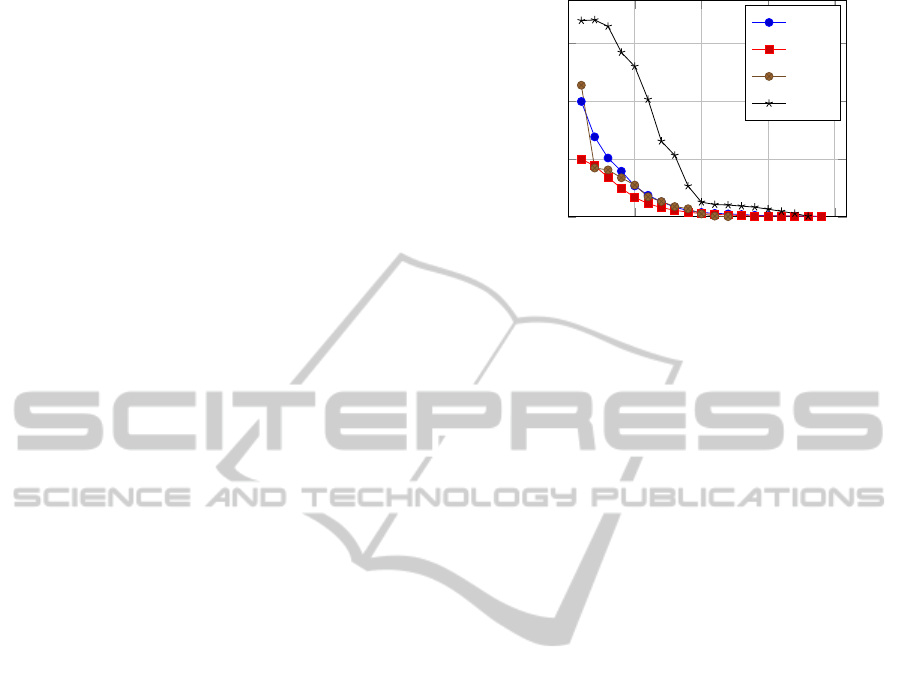
Figure 2: Energy VS iterations in the four methods, for the

ﬁrst scene element of Figure 3.

to be singled out. Like in M

, applying the function

Ω

a smooth function is obtained, whose minimum is

still located where the minimum of ρ

is located. As

in model M

this smooth function is used as velocity

to evolve the level set function, considering a general

shape for the initial guess.

Model M

. For this method we can just note that it

is the same as model M

apart from the deﬁnition of

here lacking the ﬁrst term ρ as in model M

. The

term ρ has been dropped as ρ has been used to deviate

the reference normal assigned to the domain Ω.

Finally, energy minimization with the above mod-

els amounts to use the energy function of eq. (3), and

minimizing with respect to the above deﬁned feature

based distance functions, namely:

argmin

E(Γ,ρ

(S,w)) (12)

5 IMPLEMENTATION

As previously highlighted the voxel space Ω

meaningful only for feature labeling, and for the com-

putation of the distance function ρ(S, w). Let V be

the crust of voxels close to the original input points.

For each ω

i, j,k

∈ V we deﬁne a window W (ω

i, j,k

)

of ﬁxed size and the smoothness of K

is checked

within this window. More precisely, smoothness for

each voxel in W (ω

i, j,k

) is deﬁned to be the squared

difference between the norm of the curvature gradi-

ent and the average of the curvature gradient norm

in W (ω

i, j,k

). If this value is less than a threshold τ

then the local window is accepted as smooth. The

geometric based distance function ρ

(S,w) is, then,

computed for the speciﬁed F

. Minimization is ﬁ-

nally obtained and a mesh is extracted for the selected

points. At the end all voxels close to the ﬁnal mesh

are excluded for further processing. The procedure is

GRAPP2015-InternationalConferenceonComputerGraphicsTheoryandApplications

154

Input : Unorganized point cloud S, geometric

features F(x

) = {K,h, n}, threshold τ

Output: Minimal surface energy

E (Γ, ρ

(S,w)) for each model M

i ∈ {1,2,3, 4}.

Build the voxel space Ω

⊂ Ω;

∀ w ∈ Ω

compute ρ(S,w);

F(ω

i, j,k

) = F(N (ω

i, j,k

));

V = {ω

i, j,k

| ρ(S,ω

i, j,k

) < 0.01};

while V 6= ∅ do

Select a voxel ω

i, j,k

∈ V ;

if ∀ ω

i, j,k

∈ W (ω

i, j,k



k∇K(ω

i, j,k

)k−

|W (ω

i, j,k

W (ω

i, j,k

)

k∇K(ω

i, j,k

)kdω



≤ τ

then

= F(ω

i, j,k

);

∀ w ∈ Ω

compute ρ

(S,w);

Initialize level set: φ(w,0);

Compute E (Γ, ρ

(S,w));

{ω

i, j,k

| argmin

E (Γ, ρ

(S,w))};

V = V \V

;

else

Label ω

i, j,k

∈ V as edge;

V = V \W (ω

i, j,k

);

end

Algorithm 1: Structural parts extraction.

iterated, choosing another voxel in V randomly, up to

when V is emptied. This procedure is summarized in

Algorithm 1.

As noted in Section 4, the initialization of the level

set function can use any shape, except for the ap-

proaches M

and M

. This is the main reason why the

algorithm requires many iterations to converge (see

Figure 2), as typically the starting surface lies very

far away from the input points. For the level set evolu-

tion we adopt a WENO5 approach, and the Godunov

scheme for the normal direction of motion. For sta-

bility, during evolution, the correct space derivative

(right or left), is chosen according to the sign of the

velocity of w. On the other hand the time step is de-

ﬁned according to the CLF conditions (see (Osher and

Fedkiw, 03)). We control the time step by taking only

a fraction of the maximum allowed time step. This

slows down the convergence too, though it guaran-

tees better ﬁnal results. Level set evolution is also

implemented to run on a GPU. This makes the to-

tal evolution time reasonable, but not yet useful for

real-time applications. Moreover, especially for the

models M

and M

the level set update must be eval-

uated only in the narrow band close to the interface,

and a periodic reinitialization, according to (Sussman

and Fatemi, 99), must be performed to ensure a good

reconstruction.

The proposed implementation exploits GPU to

compute the distance functions and to evolve the level

set toward its minimum. The bottleneck in computa-

tion time is given by the distance functions evaluation,

which is strongly affected by the size of S. The level

set evolution is also time expensive, but this is due to

the initialization and the chosen time step value, as

noted before.

6 EXPERIMENTS

The proposed approach has been tested with manu-

ally built point sets of simple scene elements of an

approximate size of 2 ×2 ×2 meters. This to evalu-

ate the structural component separability in terms of

planes, which are separated by their normal direction,

and have a zero curvature, as in the ﬁrst row of Figure

3. Moreover, different horizontal planes in the scene

are separated according to the h value, as in the sec-

ond row of Figure 3. The surface variation of (Pauly

et al., 03) is useful to evaluate different shapes, but it

is not enough to distinguish between a cylinder and a

sphere, but a sphere and a cone, as can be seen in the

third and fourth rows of Figure 3.

In Figure 3 the meshes extracted after level set

evolution are shown. To evaluate accuracy of the re-

construction we look at the average distance among

the vertex of the reconstructed mesh and the input

point cloud S. This distance is reported in Table 2.

One can see that the approximation of the minimal

surface energy is quite accurate. This is because the

average distance, in the most meaningful cases, is less

than a centimeter, given that the objects in Figure 3

have size of meters. A parameter which inﬂuences

this ﬁnal distance is the offset `, but only for the re-

construction models M

and M

, as the transformed

distance function γ

Ω

(B) is used in these models to

drive the level set evolution. As expected the resulting

mesh is more noisy for the model M

, but especially

for model M

as in this case the level set evolution is

governed only by H, which is smooth only very close

to the target points. This aspect is overcome in model

Table 2: Accuracy results for the four proposed models.

Both mean and max distances are reported in meters.

Mean Max Mean Max

0.007 0.035 M

0.014 0.011

0.004 0.09 M

0.021 0.21

PointCloudStructuralPartsExtractionbasedonSegmentationEnergyMinimization

155

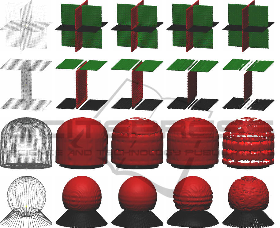
Figure 3: From left to right: results according to the four models in ascending order. Objects’ bounding box are approximately

2 ×2 ×2 meters. Number of points is approximately 10k, for each object.

, due to the addition of ρ(S,w).

Results for Gaussian added noise, with increasing

variance, are shown in Figure 4. To compute precision

and recall we consider that an input point belongs to

a segment if its distance from its closer vertex, in the

extracted mesh, is less than a threshold. Charts of

Figure 4 illustrate the results obtained increasing this

threshold. 100% of precision is obtained when the

threshold distance is quite high. On the other hand if

the noise level is low, decreasing this threshold does

not affect the good performance of precision.

7 CONCLUSIONS

The paper introduces a novel approach to the extrac-

tion of the structural parts of simple scene elements,

contextually obtaining a mesh for these parts. The

methods return a set of meshes labeled with the fea-

ture values used to extract it, and return no meshes

for points belonging to edges amid different struc-

tural parts. The main contribution is the mesh recon-

struction of singled out point clouds, despite the point

cloud is a ﬁnite set of unorganized points. Results are

accurate in general, despite the fact that the frame-

work is quite simple requiring only few parameters

for features computation. In addition, voxel size (time

step) is determined by the average density of the pro-

vided point cloud. The reported results show that the

ﬁrst and the second methods are the most accurate.

This work is a preliminary step for 3D object seg-

mentation. 3D object segmentation requires structural

parts decomposition of the unknown surface approxi-

mated by the point cloud, together with a precise parts

labeling. We cannot yet evaluate completely whether

GRAPP2015-InternationalConferenceonComputerGraphicsTheoryandApplications

156

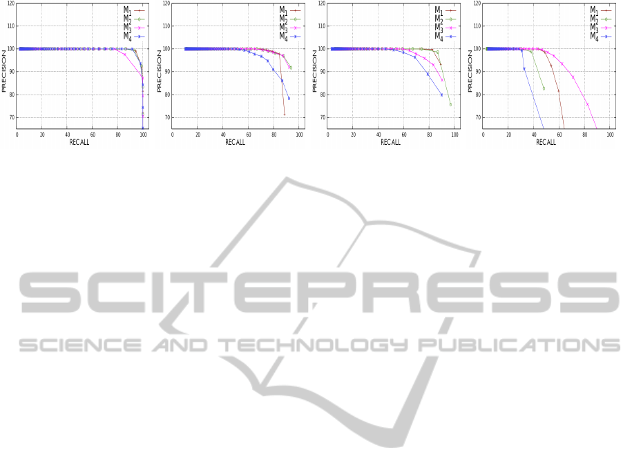
(a) σ

= 0 (b) σ

= 0.1 (c) σ

= 0.5 (d) σ

= 2

Figure 4: From Left to right: precision and recall charts for the simulated objects, for the four methods, with increasing noise.

the geometric features are sufﬁcient to single out all

the structural parts of a scene. Still, the method can be

easily extended to fulﬁl further features requirements,

adding further features in the computation of equation

(8) and (9). Also more precise geometric features,

such as the principal curvatures could provide exact

categories for structural parts.

ACKNOWLEDGEMENTS

This research is currently supported by EUFP7-ICT-

Project TRADR 60963.

REFERENCES

Golovinskiy, A. and Funkhouser, T. (’09). Min-cut based

segmentation of point clouds. In IEEE Workshop on

Search in 3D and Video (S3DV) at ICCV.

Hoppe, H., DeRose, T., Duchamp, T., Mcdonald, J., and

Stuetzle, W. (’92). Surface reconstruction from unor-

ganized points. In SIGGRAPH, pages 71–78.

Ioannou, Y., Taati, B., Harrap, R., and Greenspan, M. A.

(’12). Difference of normals as a multi-scale opera-

tor in unorganized point clouds. In 3DIMPVT, pages

501–508.

Karni, Z. and Gotsman, C. (’00). Spectral compression of

mesh geometry. In 27th Conf. on Comp. Graphics and

Int. Techniques, SIGGRAPH, pages 279–286.

Kustra, J., Jalba, A., and Telea, A. (2014). Robust segmen-

tation of multiple intersecting manifolds from unori-

ented noisy point clouds. pages 73–87.

Liang, J., Park, F., and Zhao, H. (’13). Robust and efﬁcient

implicit surface reconstruction for point clouds based

on convexiﬁed image segmentation. J. Sci. Comput.,

54(2-3):577–602.

Lloyd, S. (’06). Least squares quantization in pcm. IEEE

Trans. Inf. Theor., 28(2):129–137.

Lorensen, W. E. and Cline, H. E. (’87). Marching cubes:

A high resolution 3d surface construction algorithm.

SIGGRAPH Comput. Graph., 21(4):163–169.

Ma, T., Wu, Z., Feng, L., Luo, P., and Long, X. (’10).

Point cloud segmentation through spectral clustering.

In ICISE, pages 1–4.

Nguyen, A. and Le, B. (13). 3d point cloud segmentation:

A survey. In 6th Conf. in Robotics, Automation and

Mechatronics (RAM), pages 225–230.

Nurunnabi, A., Belton, D., and West, G. (12). Robust seg-

mentation in laser scanning 3d point cloud data. In

DICTA, pages 1–8.

Osher, S. and Fedkiw, R. (03). Level Set Methods and Dy-

namic Implicit Surfaces. Springer.

Pauly, M., Keiser, R., and Gross, M. (’03). Multi-scale fea-

ture extraction on point-sampled surfaces. Computer

Graphics Forum, 22(3):281–289.

Rusu, R. B. (’09). Semantic 3D Object Maps for Everyday

Manipulation in Human Living Environments. PhD

thesis, Computer Science dpt. TUM.

Schnabel, R., Wahl, R., and Klein, R. (’07). Efﬁcient

RANSAC for point-cloud shape detection. Comput.

Graph. Forum, 26(2):214–226.

Schreiner, J., Asirvatham, A., Praun, E., and Hoppe, H.

(’04). Inter-surface mapping. SIGGRAPH, pages

870–877, NY, USA. ACM.

Shamir, A. (08). A survey on mesh segmentation tech-

niques. Comput. Graph. Forum, 27(6):1539–1556.

Sussman, M. and Fatemi, E. (’99). An efﬁcient, interface-

preserving level set redistancing algorithm and its

application to interfacial incompressible ﬂuid ﬂow.

SIAM J. Sci. Comput., 20(4):1165–1191.

Tran, T., Cao, V., Nguyen, V., Ali, S., and Laurendeau, D.

(’14). Automatic method for sharp feature extraction

from 3d data of man-made objects. In GRAPP 2014,

pages 112–119.

Turner, E. and Zakhor, A. (’14). Floor plan generation

and room labeling of indoor environments from laser

range data. In GRAPP 2014, pages 22–33.

Wirjadi, O. (07). Survey of 3d image segmentation meth-

ods. Technical Report 123, Fraunhofer (ITWM).

Zhao, H. K., Stanley, O., Barry, M., and Myungjoo, K.

(’98). Implicit, nonparametric shape reconstruction

from unorganized points using a variational level set

method. Computer Vision and Image Understanding,

80:295–319.

Zhao, H. K., Stanley, O., and Ronald, F. (’01). Fast surface

reconstruction using the level set method. In IEEE

Workshop on Variational and Level Set Methods in

Computer Vision, pages 194–201.

PointCloudStructuralPartsExtractionbasedonSegmentationEnergyMinimization

157