
Point-wise Diversity Measure and Visualization for Ensemble of
Classifiers
With Application to Image Segmentation
Ahmed Al-Taie
1,3
, Horst K. Hahn
1,2
and Lars Linsen
1
1
Jacobs University, Bremen, Germany
2
Fraunhofer MEVIS, Bremen, Germany
3
Computer Science Department, College of Science for Women, Baghdad University, Baghdad, Iraq
Keywords:
Ensemble of Classifiers, Image Segmentation, Diversity.
Abstract:
The idea of using ensembles of classifiers is to increase the performance when compared to applying a single
classifier. Crucial to the performance improvement is the diversity of the ensemble. A classifier ensemble
is considered to be diverse, if the classifiers make no coinciding errors. Several studies discuss the diversity
issue and its relation to the ensemble accuracy. Most of them proposed measures that are based on an ”Oracle”
classification. In this paper, we propose a new probability-based diversity measure for ensembles of unsuper-
vised classifiers, i.e., when no Oracle machine exists. Our measure uses a point-wise definition of diversity,
which allows for a distinction of diverse and non-diverse areas. Moreover, we introduce the concept of further
categorizing the diverse areas into healthy and unhealthy diversity areas. A diversity area is healthy for the
ensemble performance, if there is enough redundancy to compensate for the errors. Then, the performance
of the ensemble can be based on two parameters, the non-diversity area, i.e., the size of all regions where the
classifiers of the ensemble agree, and the healthy diversity area, i.e., the size of the regions where the diversity
is healthy. Furthermore, our point-wise diversity measure allows for an intuitive visualization of the ensemble
diversity for visual ensemble performance comparison in the context of image segmentation.
1 INTRODUCTION
In pattern recognition and machine learning, several
studies confirmed the concept that combining the re-
sults of multiple classifiers can yield more reliable
and accurate results when compared to the results
of a single classifier (Kittler et al., 1998; Sharkey,
1999; Dietterich, 2000; Kuncheva, 2004; Fred and
Jain, 2005). This concept is known as committee ma-
chine, mixture of experts, or ensemble of classifiers
(Mignotte, 2010). An important aspect of establishing
ensembles is the diversity such that complementary
information of individual classifiers can be combined
to improve the final result. An ensemble of classifiers
is said to be diverse, if the classifiers make no coincid-
ing errors. Diversity can be achieved through several
approaches: Several instances of the same algorithm
can be applied on different subsets of the input data
or on the same data but initialized using different pa-
rameter settings. Diversity can also be achieved either
using different representations of the data (e.g., using
the same input image represented in different color
spaces), or using different algorithms with sufficiently
diverse behaviors on the input data (Fred and Jain,
2005; Mignotte, 2010). Another important issue is the
ensemble redundancy (or knowledge redundancy) as-
suring that the individual classifiers (or experts) share
their knowledge in order to make a more accurate
decision. In the context of combining the results of
classifiers within an ensemble, there have been sev-
eral combining strategies proposed in the literature.
Examples of strategies are majority votes, weighted
majority votes, or probability rules such as product,
sum, maximum, minimum, median, etc. The majority
votes, weighted majority votes, and sum rules, where
the individual classifiers contribute to the final ensem-
ble decision, are the most commonly used rules. In
general, the concept of ensembles of classifiers was
mostly used in machine learning applications for su-
pervised classification. The main focus of the re-
searchers in the field is on the diversity definition and
its evaluation (Kuncheva, 2004; Masisi et al., 2008),
while the ensemble redundancy is mostly omitted in
the discussion. Diversity and redundancy are some-
569
Al-Taie A., Hahn H. and Linsen L..
Point-wise Diversity Measure and Visualization for Ensemble of Classifiers - With Application to Image Segmentation.
DOI: 10.5220/0005309605690576
In Proceedings of the 10th International Conference on Computer Vision Theory and Applications (VISAPP-2015), pages 569-576
ISBN: 978-989-758-089-5
Copyright
c
2015 SCITEPRESS (Science and Technology Publications, Lda.)

what conflicting concepts and a desired diversity is a
diversity that, at the same time, has sufficiently large
redundancy. This explains why most of the proposed
diversity measures fail in defining a strong relation
between the ensemble diversity and its accuracy. The
desired diversity requests that, if a subset of the en-
semble classifiers make errors at some point, the re-
maining classifiers in the ensemble should make cor-
rect decisions to allow for a correction. For an en-
semble to be robust, the number of correct decisions
should be more than the number of erroneous deci-
sions (at each point). Such a diversity is the main mo-
tivation behind the concept of ensemble of classifiers
methods. Thus, since the diversity is the most im-
portant ensemble property, several diversity measures
have been proposed for different ensemble design ap-
plications. Kuncheva (Kuncheva, 2004) reviewed ten
diversity measures and presented several applications
of diversity measures in ensemble design, thinning,
evaluation, and selection. However, all these mea-
sures of diversity require the availability of a ground-
truth (or Oracle) classification, which is not always
available (especially for unsupervised learning).
In this paper we distinguish between two types of
the ensemble diversity and refer to them as healthy
and unhealthy diversity. A diversity area is healthy,
iff, in addition to the diversity, enough redundancy
exists to compensate for the errors.
For the distinction between healthy and unhealthy
diversity areas, we propose a new point-wise diversity
measure, which is a non-pairwise measure able to es-
timate the diversity of the ensemble classifiers (or any
subset of classifiers) in the absence of ground truth
(i.e., it is suitable for unsupervised classification), see
Section 3. Based on a certain threshold, the healthy
and unhealthy diversity areas are computed, see Sec-
tion 4. Our new diversity measure can be used for
designing the ensemble classifiers or for estimating
the ensemble performance, cf. (Kuncheva, 2004; Ma-
sisi et al., 2008). Furthermore, when applied to image
segmentation, the point-wise definition of our diver-
sity measure allows for an ensemble diversity visual-
ization, which supports visual ensemble performance
comparisons, see Section 5.
The contributions of our paper can be summarized
as: (1) Defining a point-wise diversity measure for
ensembles, which allows for the definition of healthy
and unhealthy diversity regions. (2) Visual represen-
tation and analysis of diversity measures. (3) Diver-
sity computation without known ground truth, i.e., it
is applicable to unsupervised classification.
Our application domain is medical image seg-
mentation. Thus, we applied the proposed methods
on a synthetic image that mimics the properties of
main brain tissues in a T1-weighted MR image cor-
rupted with mixed noise, and on the simulated MR
images from Brainweb (MNI, 1997) corrupted with
5% Gaussian noise and 20% Intensity non-uniformity.
The synthetic and the simulated data with known
ground truth allow for the computation of segmenta-
tion accuracy to evaluate our methods, see Section 6
for the experimental set-up and Section 7 for results
and discussion.
2 RELATED WORK
In recent years, combining ensemble of simple clas-
sifiers in order to improve their performance has wit-
nessed a great attention by researchers across diverse
fields to solve different classification problems (Kit-
tler et al., 1998; Dietterich, 2000; Mignotte, 2010;
Fred and Jain, 2005; Paci et al., 2013; Artaechevar-
ria et al., 2009; Langerak et al., 2010). The ensemble
diversity (or error diversity) issue and its relation to
the ensemble accuracyattract the most interesting dis-
cussion in this concept (Kuncheva, 2004; Kuncheva
and Whitaker, 2003). In this paper, we propose a new
diversity measure suitable for ensembles of unsuper-
vised classifiers (i.e., in the absence of ground truth).
In addition to the importance of diversity for the im-
provement of ensemble performance, the diversity
measure is also useful for several classifier ensem-
ble applications such as ensemble diversity visualiza-
tion, ensemble overproduceand select, or diversity for
building ensembles (for more details see the diversity
chapter in (Kuncheva, 2004)). Kuncheva (Kuncheva,
2004) reviewed ten pairwise and non-pairwise diver-
sity measures, but all depend on the availability of
ground truth (or Oracle) classification, which is not
always provided. Another issue with pairwise mea-
sures is their complexity. To get a single value for
ensemble diversity, the average across all pairwise di-
versity values needs to be calculated (i.e., L(L− 1)/2
pairs for an ensemble of size L).
The point-wise property for our proposed mea-
sure enables us to estimate the local diversity and,
consequently, to distinguish among different levels
of diversities (i.e., to distinguish between the desired
(healthy) and undesired (unhealthy) diversity area for
an ensemble of classifiers to be more robust). The
diversity measures proposed by Masisi et al. (Ma-
sisi et al., 2008) and Sirlantzis et al. (Sirlantzis et al.,
2008) are the closest diversity measures to our pro-
posed measure. However, the two measures like
the previous measures are global measures (i.e., not
point-wise) and, consequently, by computing the av-
erage diversity one loses the internal distribution of
VISAPP2015-InternationalConferenceonComputerVisionTheoryandApplications
570

the diversity levels in the ensemble. Sirlantzis et al.
(Sirlantzis et al., 2008) use k statistics to produce
value 0 for no diversity and 1 for maximum diversity.
The measure by Masisi et al. (Masisi et al., 2008) as-
signs with each individual classifier (for an ensemble
of 21 classifiers) the probability that the classifier is
selected in the ensemble out of 120 individual clas-
sifiers. Based on these probabilities, the entropy is
used to measure the diversity of an ensemble. Then,
a genetic algorithm that uses the diversity value as fit-
ness function is used to select the best ensemble of
size 21 out of 120 classifiers. It is clear that Masisi
et al.’s measure is particularly designed for this sys-
tem and not generally applicable for different ensem-
ble designs and applications as the used probabilities
are not related to the error probabilities of the individ-
ual classifiers.
The problem of medical image segmentation has
been addressed in the framework of ensemble of
classifiers methods using several atlas-based segmen-
tations or several human rater segmentations. As
pointed out in (Rohlfing and Maurer, 2005), produc-
ing multiple atlases is time consuming and tedious.
Thus such atlases are not always available. Langerak
et al. (Langerak et al., 2010) referred to the shortcom-
ing of atlas-based segmentations as being an equiv-
alent to segmentation by human expert. They also
discussed two important drawbacks of using multi-
ple atlases, namely, the large computational costs of
the registration process and the shape variance in the
atlas ensemble that is not always similar to that of
the population from which the input image is drawn.
These drawbacks may lead to the ensemble methods
that use atlas-based segmentations to be impractical.
Although Langerak et al. (Langerak et al., 2010) tried
to reduce the effects of these drawbacks by reducing
the number of atlases through an atlas selection pro-
cedure, the problem is only alleviated and not solved.
To avoid such drawbacks, we propose to combine the
results of several automatic segmentations of the tar-
get image with acceptable accuracies instead of com-
bining the results of registering several atlases to the
target image. The diversity is achieved through ap-
plying several unsupervised segmentation algorithms
that use different approaches under the assumption
that the probability that different approaches (with
high or acceptable average accuracy, e.g., > 0.80%)
produce the same errors is very low.
3 POINT-WISE DIVERSITY
The proposed diversity measure is based on the proba-
bility of classes that appear in the ensemble decisions
using the normalized entropy to produce a value be-
tween 0 (no diversity)and 1 (maximumdiversity). We
choose to use the normalized entropy of the classes
probabilities, as it is easy to compute, its value re-
flects both the degree of agreement and the error rate
of the individual classifiers (assuming that sufficiently
accurate individual classifiers mostly agree on cor-
rect decisions), and it allows for both point-wise and
global diversity evaluation. The point-wise property
for the proposed measure enables us to estimate the
local diversity and consequently to distinguish among
different levels of diversities. Based on this flexibility,
a new diversity view is introduced, which is able to
distinguish three diversity areas: (1) the non-diversity
area, where all individualclassifiers agree on the same
decision (which can be assumed to be the correct de-
cision if the individual classifiers have high accura-
cies); (2) the healthy diversity area, where most of
the individual classifiers agree on the same decision;
(3) the unhealthy diversity area, where two or more
classes haveapproximately similar probabilitiesin the
ensemble decisions (i.e., when the uncertainty in the
ensemble is high). Following this train of thoughts,
the local diversity D(P
v
), i.e., the diversity at point v
with the probability vector P
v
(which represents the
probability distribution for all classes in the individ-
ual classifier’s output at that point) is given by the nor-
malized entropy:
D(P
v
) = H(P
v
)/log
2
(c), (1)
where H(P
v
) is the entropy of the probability vec-
tor P
v
(H(P
v
) = −
∑
c
i=1
P
v
i
log
2
P
v
i
), c the number of
classes, and log
2
(c) the normalization term. Based
on the local diversity, the global diversity D(I
en
) for
the entire ensemble image (or dataset) I
en
can be eval-
uated by
D(I
en
) =
1
N
∑
v∈I
en
D(P
v
), (2)
where N is the image cardinality |I
en
|.
The local diversity is 0 when all classifiers agree
on one decision and it is 1 when all classes have equal
probability. Otherwise, the measure has values in
the interval (0,θ) with θ ≤ 0.5 when one class domi-
nates over others and has values in the interval [θ,1)
when two or more classes have mostly similar prob-
abilities in the ensemble decisions. The philosophy
of the measure is to distinguish between two types
of diversity: healthy diversity and unhealthy diver-
sity. The healthy diversity (for a robust ensemble)
is located in the interval [0,θ) where the probability
of errors is low, while the unhealthy diversity is lo-
cated in the interval [θ, 1], where the probability of er-
rors is high. The selection of threshold θ depends on
the number of classes and how large the proportion
Point-wiseDiversityMeasureandVisualizationforEnsembleofClassifiers-WithApplicationtoImageSegmentation
571

of the dominating class is in the ensemble decision
for a certain point to be considered in the healthy di-
versity interval. For example, when assuming that a
point belongs to the healthy area iff. more than 81%
of individual classifiers agree on the same decision,
we choose θ = 0.35 for c = 4. This follows the ob-
servation that the normalized entropy of the vector
(0.811,0.199,0,0) is 0.349687, while the normalized
entropy of the vector (0.8,0.2,0,0) is 0.360964.
This philosophy is based on a heuristic assump-
tion that the ensemble consists of a set of individual
classifiers with acceptable accuracy (e.g., ≥ 0.80%).
If this is the case, then the probability that all (or most
of) the classifiers agree on a wrong decision is very
low and, consequently, there would be a low error
rate on the final ensemble decision. Conversely, in
the unhealthy interval, the probability of individual
errors increases when two or more classes have sim-
ilar probabilities. Even though the true class is most
likely one of the reported classes, the probability of
having an error ensemble decision is still high. Un-
der this interpretation, the majority votes combining
strategy where the winner class is the one receiving
the largest number of votes in the classifier ensemble
(Kittler et al., 1998) is very correlated to our diversity
measure.
The proposed diversity measure can be helpful
to locally select at each point the suitable combin-
ing strategy for each interval of diversity values or
to globally evaluate the entire ensemble diversity
whether it is healthy or unhealthy in addition to other
diversity applications (see (Kuncheva, 2004)).
4 DIVERSITY REGIONS
According to our diversity concept, two global di-
versity areas, the non-diversity area NDA and the di-
versity area DA, can be defined to evaluate the en-
semble performance as follows: DA =
∑
v∈I
en
δ
v
, and
NDA = N − DA, where δ
v
is the binary function
δ
v
=
1 if D(P
v
) > 0
0 otherwise,
(3)
and N is the image cardinality |I
en
|.
For further ensemble evaluation, the diversity area
can be subdivided into the healthy diversity area HDA
and the unhealthy diversity area UDA as follows:
HDA = |{v ∈ D
A
∧ D(P
v
) < θ}| and UDA = DA −
HDA, where D
A
is the set of points in the diversity
area DA.
The diversity density DD can be calculated for
the diversity area and its parts the healthy and un-
healthy diversity areas densities (HDD and UDD) as
follows: DD =
∑
v∈D
A
D(P
v
)
DA
, HDD =
∑
v∈HD
A
D(P
v
)
HDA
,
and UDD =
∑
v∈UD
A
D(P
v
)
UDA
, where HD
A
and UD
A
are
the sets of points in the healthy (HDA) and unhealthy
diversity areas (UDA), respectively.
The non-diversity ratio NDR, diversity ratio DR,
the healthy diversity ratio HDR, and unhealthy di-
versity ratio UDR are given by: NDR = NDA/N,
DR = DA/N, HDR = HDA/N, and UDR = UDA/N,
respectively.
Then, the ensemble diversity evaluation can be
based on two parameters, namely, the non-diversity
area NDA (or NDR), as it represents the area of all
individual classifiers’ agreement (on the correct de-
cision mostly), and the healthy diversity area HDA
(or HDR), where the probability for an ensemble in
producing the correct decision is very high. Assum-
ing that individual classifiers have a sufficiently high
accuracy, the non-diversity and the healthy diversity
areas are expected to cover a large amount of points
with correct decisions mostly. Consequently, ensem-
bles with larger non-diversity area and larger healthy
diversity area perform better.
5 DIVERSITY VISUALIZATION
In addition, we propose a point-wise diversity visual-
ization that can be useful for visual diversity compar-
ison in the context of image segmentation. We pro-
pose a color mapping of the identified areas in the
image domain, potentially overlaid with the original
input images. Two color maps are being proposed,
a categorical one and a categorical with color transi-
tions within each category. In the first visualization
method, the different diversity areas are color-coded
using three distinct colors (black: non-diversity area,
blue: healthy diversity area, and red: unhealthy diver-
sity area). In the second visualization method, the in-
ternal diversity level of the healthy and unhealthy di-
versity areas are color-coded using a continuous tran-
sition between two colors for each area. The healthy
diversity area gradually changes from dark blue to
light blue, while the unhealthy diversity area grad-
ually changes from red to yellow (the non-diversity
area remains black). The proposed discrete and con-
tinuous color-coding can be overlaid with the origi-
nal image by assigning to the non-diversity pixels the
original intensities instead of the black color. Exam-
ples are given in the subsequent sections.
VISAPP2015-InternationalConferenceonComputerVisionTheoryandApplications
572

6 EXPERIMENTAL SET-UP
As we mentioned above, to avoid the drawbacks of
combining several atlas-based segmentations, we pro-
posed to combine the results of several unsupervised
segmentations. In this paper, we use several variants
of the fuzzy c-means (FCM) algorithm introduced by
Bezdek (Bezdek, 1981). Fuzzy c-means is one of the
most commonly used algorithms for image segmen-
tation (Mohamed et al., 1999; Chen S., Zhang D.,
2004; Zhang and Chen, 2004; Chuang et al., 2006;
Ahmed et al., 2002; Yuan et al., 2005). The FCM vari-
ants used in this paper are: (1) the modified fuzzy c-
means (mFCM) (Mohamed et al., 1999), (2) the Bias-
corrected FCM (BCFCM) (Ahmed et al., 2002) and
an improved version thereof, (3) the Bias-corrected
FCM with weighted α (BCFCM
WA) (Yuan et al.,
2005), (4) the spatial fuzzy c-means (sFCM) (Chuang
et al., 2006), (5) the spatial kernelized fuzzy c-means
(SKFCM) ( Chen S., Zhang D., 2004; Zhang and
Chen, 2004), (6) the simplified fuzzy c-means method
(FCMS1) using mean filter ( Chen S., Zhang D.,
2004), (7) the CLIC algorithm (Li, C. and Xu, C. and
Anderson, A. and Gore, J., 2009), and finally (8) the
fuzzy rule based system (FRBS) (Tolias and Panas,
1998).
(a) (b)
Figure 1: (a) synthetic image corrupted with mixed noise.
(b) simulated T1-weighted MRI corrupted with noise.
In the subsequent section, we present and com-
pare the experimental results of applying the proposed
methods on the synthetic images in Figure 1(a), and
on the simulated T1-weighted MRI in Figure 1(b).
For the synthetic image, we tried to mimic the main
brain tissues of MR T1- and T2-weighted images
in a synthetic image (i.e., the background Bg, the
white matter WM, the gray matter GM, and the cere-
brospinal fluid CSF). We generate an example of four
respective classes with complex structures as shown
in Figure 1(a). We corrupted our synthetic image with
different types of noise that are common in medical
data such as Gaussian, salt-and-pepper, or sinusoidal
noise. In first experiment, we use a synthetic image
corrupted with a mixture of the three types of noise
Table 1: Segmentation accuracy (SA) in percentage for the
synthetic image in Figure 1(a) when applying the modified
FCM variants methods that we use as the individual classi-
fiers to assemble the ensemble.
Method SA% Method SA%
BCFCM 85.33 FCMS1 98.5565
CLIC 88.8062 FRBS 98.5657
SKFCM 94.0079 mFCM 98.7747
BCFCM WA 94.30 sFCM 99.388
as shown in Figure 1(a). Before describing the exper-
iments, we show in Table 1 the segmentation accu-
racy for each of the above FCM variants (individual
classifiers). The segmentation accuracy that is used
throughout this paper is given by
SA =
|correctly classified pixels|
Total number of pixels
× 100%. (4)
As our experimental results showed that the ma-
jority votes rule almost always achieved the best per-
formance in terms of segmentation accuracy and due
to its relation to the proposed diversity measure, we
use it as the combining strategy in our experiments in
the results and discussion section. The majority votes
rule selects the class that has been reported the most
by the individual classifiers as the combined classifi-
cation result.
7 RESULTS AND DISCUSSION
In our experiments, we apply the proposed diversity
measures, the diversity areas ratios, and the diver-
sity densities on five ensembles with different sizes
(4,5,6,7,7). The experiments confirm our discussion
on the proposed diversity measure and the healthy
and unhealthy diversity areas. Figure 2(a) shows the
majority rule (MajR) segmentation accuracy(SA),and
the different diversity areas ratios (NDR, DR, HDR,
and UDR). Figure 2(b) shows the misclassified ratios
(NDA MR, DA MR, HDA MR, and UDA MR) of the
different diversity areas regarding the corresponding
diversity areas. Figure 2(c) shows the diversity den-
sity of the different diversity areas (DD, HDD, and
UDD). The sizes of ensembles from Ens
1 to Ens 5
are 4,5,6,7, and 7, respectively. We start with an en-
semble of size 4 (BCFCM, BCFCM
WA, SKFCM,
and FCMS1). Then, we add a fifth classifier FRBS
for Ens
2, add a sixth classifier sFCM for Ens 3, and
add a seventh classifier mFCM for Ens 4. Finally, for
Ens 5, we take Ens 4 and replace sFCM with CLIC.
The first four experiments show that the NDR for the
ensembles are approximately equal and that the per-
formance of the ensembles with larger healthy diver-
sity area (HDA) is better. While the non-diversity
Point-wiseDiversityMeasureandVisualizationforEnsembleofClassifiers-WithApplicationtoImageSegmentation
573

ratios are approximately similar for ensembles Ens 1
and Ens 2, the healthy diversity area is zero for Ens 1
and the accuracy (SA) increases as the size of en-
sembles increases (from Ens
2 to Ens 1). This is in-
dicated by the increase of the performance of UDA
(reduced UDA MR for Ens
2), although UDA was
similar for both ensembles. The same behavior or
trend can be seen when adding even more classifiers
in Ens
3 and Ens 4. The misclassified ratio UDA MR
is steadily decreasing.
In general, we judge the performanceof an ensem-
ble by first inspecting the non-diversity area where
the ensemble with the larger non-diversity area (all
classifiers agree in those areas) typically leads to bet-
ter segmentation accuracy. If the non-diversity area
is comparable, then the ensemble with larger healthy
diversity area (HDA) shall be preferred, as there is a
higher chance of compensating for the error and mak-
ing the right decision. If the healthy diversity area for
two ensembles is also comparable (as in Ens 1 and
Ens
2 or in Ens 3 and Ens 4), then we inspect the di-
versity density of the diversity areas: The ensemble
with lower density (especially in the UDA) has better
accuracy.
Comparing the results of Ens
4 and Ens 5, where
we exchanged the individual classifier with best accu-
racy (99.3%)with a low-accuracyclassifier (88%), we
can observe that the accuracy was not affected very
much, even though the NDR is decreased by 8%. This
can be explained by observing that the healthy area
increased, i.e., the lower accuracy estimates could be
compensated.
In Figure 2(b), we can observe that most of the
misclassified ratios are in the unhealthy diversity area,
while the non-diversity and healthy diversity areas
have very small error ratios. This finding confirms
that our diversity measures are indeed suitable and ap-
propriate.
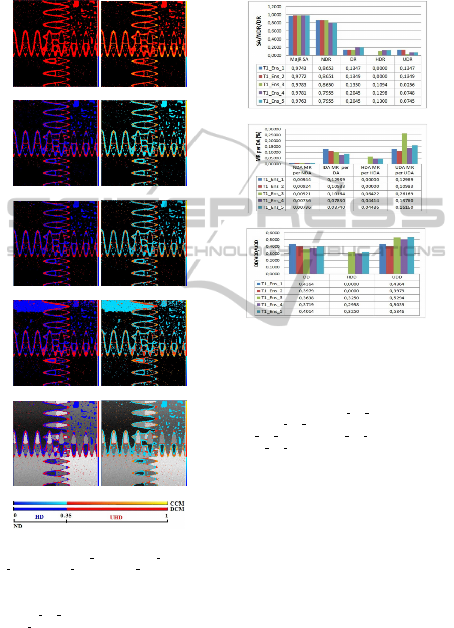
Figure 3 shows examples of the proposed visual
encoding of the ensemble diversity areas. The exam-
ples relate to the experiments shown in Figure 2. The
first column shows the purely categorical color map-
ping while the second column shows the color map-
ping with continuous two-color transitions per cate-
gory. The images show the following ensembles: (a
and b) the second ensemble (Ens
2), (c and d) the
third ensemble (Ens 3), (e and f) the fourth ensem-
ble (Ens
4), (g and h) fifth ensemble (Ens 5), and
(i and j) fourth ensemble (Ens 4) again but overlaid
with the original image in non-diversity areas. Figure
3(k) shows the legends of the discrete color mapping
(DCM) and the continuous color mapping (CCM) that
were used to visualize the healthy (HD) and unhealthy
(UD) diversity areas. We can observe that in the en-
(a)
(b)
(c)
Figure 2: (a) The segmentation accuracy (SA) with the
(non-diversity(ND), diversity(D), healthy diversity(HD),
and unhealthy diversity(UD)) ratios; (b) their misclassified
ratios (MR), and (c) their diversity densities (DD) compari-
son for ensembles of different sizes on the synthetic image.
semble of Figure 3(a) only unhealthy diversity areas
exist, while for the ensemble in Figure 3(c) parts of
the unhealthy diversity area converted to healthy di-
versity areas (the blue area). Some scattered healthy
points in Figure 3(c) (Ens
3) become unhealthy in
Figure 3(e), which explains the increment of UDA in
the fourth ensemble (Ens
4), cf. Figure 2. In general,
the visualizations allow for a quick overview compar-
ison of the quality of the chosen ensembles and for
a more detailed visual analysis on which areas cause
problems.
To further validate the proposed methods, we ap-
plied them to simulated MR brain images (MNI,
1997). In Figure 4, we show the results for T1-
weighted images corrupted with 5% Gaussian noise
and 20% intensity non-uniformity shown in Fig-
ure 1(b). In this experiment, we compare the re-
sults of five ensembles (T1 Ens 1-T1 Ens 5) with
VISAPP2015-InternationalConferenceonComputerVisionTheoryandApplications
574
(a) (b)
(c) (d)
(e) (f)
(g) (h)
(i) (j)
(k)
Figure 3: The proposed diversity visualizations for the ex-
periments in Figure 2. Ens 2 (a) and (b), Ens 3 (c) and (d),
Ens
4 (e) and (f), Ens 5 (g) and (h), Ens 4 (i) and (j), (k) the
legend.
sizes (4,5,6,7, and 6), respectively. The first en-
semble T1
Ens 1 consists of 4 classifiers (CLIC,
BCFCM WA, FCMS1, and FRBS). Then, we add a
(a)
(b)
(c)
Figure 4: (a) The segmentation accuracy (SA) with the
(non-diversity(ND), diversity(D), healthy diversity(HD),
and unhealthy diversity(UD)) ratios; (b) their misclassified
ratios (MR), and (c) their diversity densities (DD) compar-
ison for ensembles of different sizes on the simulated MRI
of Figure 1(b).
fifth classifier mFCM for T1
Ens 2, a sixth classifier
sFCM for T1 Ens 3, and a seventh classifier SKFCM
for T1
Ens 4. Finally, for T1 Ens 5 we removesFCM
from T1 Ens 4. Figure 4 shows the diversity areas
for these ensembles, their misclassified ratios, diver-
sity densities, and segmentation accuracies. We can
observe a similar behavior in the performance of the
ensembles to the one we observed when investigating
the synthetic image. Hence, similar conclusions can
be drawn.
8 CONCLUSIONS
In recent years, the concept of combining several clas-
sifiers in order to produce classification accuracy that
outperforms the accuracy of the individual classifiers
attracted the attention of researchers in different fields
to improve the segmentation accuracy or to evaluate
Point-wiseDiversityMeasureandVisualizationforEnsembleofClassifiers-WithApplicationtoImageSegmentation
575

the performance level of the individual segmentation.
We proposed a novel probability-based diversity mea-
sure with a new concept that is suitable for unsuper-
vised classifiers. In this concept, we distinguish be-
tween healthy and unhealthy diversity areas for an
ensemble design. The experimental results show the
appropriateness of our approach and how it can be
used to evaluate the performance of ensembles. We
also proposed a color-coded diversity visualization to
visually encode the healthy and unhealthy diversity
areas and their diversity level. This means that the
diversity visualization can be used in comparing the
performance of different ensembles.
REFERENCES
Chen S., Zhang D. (2004). Robust image segmentation us-
ing fcm with spatial constraints based on new kernel-
induced distance metric. IEEE Trans. on System, Man
and Cybernetics-Part B, 34(4):1907–1916.
Ahmed, M. N., Yamany, S. M., Mohamed, N., Farag, A. A.,
and Moriarty, T. (2002). A modified fuzzy c-means
algorithm for bias field estimation and segmentation
of mri data. IEEE Transactions on Medical Imaging,
21(3):193–199.
Artaechevarria, X., Muoz-Barrutia, A., and de Solorzano,
C. O. (2009). Combination strategies in multi-atlas
image segmentation: Application to brain mr data.
IEEE Transactions Medical Imaging, 28(8):1266–
1277.
Bezdek, J. (1981). Pattern recognition with fuzzy objective
function algorithms. Plenum, NY.
Chuang, K.-S., Tzeng, H.-L., Chen, S., Wu, J., and Chen,
T.-J. (2006). Fuzzy c-means clustering with spatial
information for image segmentation. Computerized
Medical Imaging and Graphics, 30(1):9 – 15.
Dietterich, T. G. (2000). Ensemble methods in machine
learning. In Proceedings of the First International
Workshop on Multiple Classifier Systems, pages 1–15,
London, UK, UK. Springer-Verlag.
Fred, A. and Jain, A. (2005). Combining multiple clus-
terings using evidence accumulation. Pattern Analy-
sis and Machine Intelligence, IEEE Transactions on,
27(6):835–850.
Kittler, J., Hatef, M., Duin, R. P. W., and Matas, J. (1998).
On combining classifiers. Pattern Analysis and Ma-
chine Intelligence, IEEE Transactions on, 20(3):226–
239.
Kuncheva, L. I. (2004). Combining Pattern Classifiers:
Methods and Algorithms. Wiley-Interscience.
Kuncheva, L. I. and Whitaker, C. J. (2003). Measures
of diversity in classifier ensembles and their relation-
ship with the ensemble accuracy. Machine learning,
51(2):181–207.
Langerak, R., van der Heide, U. A., Kotte, A. N. T. J.,
Viergever, M. A., van Vulpen, M., and Pluim, J. P. W.
(2010). Label fusion in atlas-based segmentation us-
ing a selective and iterative method for performance
level estimation (simple). IEEE Transactions Medical
Imaging, 29(12):2000–2008.
Li, C. and Xu, C. and Anderson, A. and Gore, J. (2009). Mri
tissue classification and bias field estimation based on
coherent local intensity clustering: A unified energy
minimization framework. In Information Processing
in Medical Imaging, volume 5636 of Lecture Notes
in Computer Science, pages 288–299. Springer Berlin
Heidelberg.
Masisi, L. M., Nelwamondo, F. V., and Marwala, T. (2008).
The use of entropy to measure structural diversity.
CoRR, abs/0810.3525.
Mignotte, M. (2010). A label field fusion bayesian model
and its penalized maximum rand estimator for image
segmentation. IEEE Transactions on Image Process-
ing, 19(6):1610–1624.
MNI (1997). Brainweb, simulated brain
database, available since 1997. Available at
http://www.bic.mni.mcgill.ca/brainweb/, access time:
on November 2012.
Mohamed, N., Ahmed, M., and Farag, A. (1999). Modified
fuzzy c-mean in medical image segmentation. In Pro-
ceedings IEEE International Conference on Acous-
tics, Speeeh, and Signal Processing, 1999, Piscat-
away, NI USA, volume 6, pages 3429–3432 vol.6.
Paci, M., Nanni, L., and Severi, S. (2013). An ensemble
of classifiers based on different texture descriptors for
texture classification. Journal of King Saud University
- Science, 25(3):235 – 244.
Rohlfing, T. and Maurer, C. R. J. (2005). Multi-classifier
framework for atlas-based image segmentation. Pat-
tern Recognition Letters, 26(13):2070 – 2079.
Sharkey, A. J. C. (1999). Combining artificial neural nets:
ensemble and modular multi-net systems. Springer-
Verlag, New York.
Sirlantzis, K., Hoque, S., and Fairhurst, M. (2008). Diver-
sity in multiple classifier ensembles based on binary
feature quantisation with application to face recogni-
tion. Applied Soft Computing, 8(1):437 – 445.
Tolias, Y. and Panas, S. (1998). On applying spatial
constraints in fuzzy image clustering using a fuzzy
rule-based system. Signal Processing Letters, IEEE,
5(10):245–247.
Yuan, K., Wu, L., Cheng, Q., Bao, S., Chen, C., and Zhang,
H. (2005). A novel fuzzy c-means algorithm and its
application. International Journal of Pattern Recog-
nition and Artificial Intelligence, 19(8):1059–1066.
Zhang, D. and Chen, S. (2004). A novel kernelised fuzzy
c-means algorithm with application in medical im-
age segmentation. Artificial Intelligence in Medicine,
32(1):37–50.
VISAPP2015-InternationalConferenceonComputerVisionTheoryandApplications
576
