
Computing Corpus Callosum as Biomarker for Degenerative Disorders
Thomas Kovac, Sammy Rogmans and Frank Van Reeth
Expertise Centre for Digital Media, Hasselt University - tUL - iMinds, Wetenschapspark 2, 3590 Diepenbeek, Belgium
Keywords:
Biomarker, Corpus Callosum, Image Registration, GPGPU, CUDA.
Abstract:
The developed framework can automatically extract a plane with minimal corpus callosum area while simul-
taneously segmenting it. The method used, introduced by Ishaq, treats the corpus callosum area as a function
of the plane extraction parameters and it uses deformable registration to generate a displacement field that
can be used for the calculation of the corpus callosum area. Our registration framework is accelerated using
CUDA, which enables researchers to benchmark huge amounts of data (patients) to test the hypothesis of the
corpus callosum evolution as a biomarker for multiple degenerative disorders like e.g. Alzheimer disease and
multiple sclerosis (MS).
1 INTRODUCTION
Multiple Sclerosis (MS) is an inflammatory disorder
of the brain and spinal cord and it has been known
to cause atrophy and deformation in the corpus cal-
losum. Longitudinal studies try to quantify these
changes by using medical image analysis techniques
for measuring and analyzing the size and shape of the
corpus callosum. These medical techniques mostly
analyze and track changes in the corpus callosum by
measuring the cross-sectional area by selecting a 2-
D measuring plane, typically the midsagittal plane.
If this identification is done incorrectly, the measure-
ment of the corpus callosum area will also be faulty.
Therefore, an automation of finding a plane with min-
imal corpus callosum area is implemented to ensure
that the measurement of the cross-sectional area is
done correctly with high accuracy.
The employed method of finding a plane with
minimal corpus callosum area depends heavily on de-
formable image registration. As the image registra-
tion process must be performed multiple times, it is
important that the registration is performed as quickly,
and correctly, as possible. The use of a GPU greatly
improves computation time, so this framework is built
out of algorithms and data structures that exploit its
parallel computation capabilities and hardware. The
implemented framework is algorithmically inspired
by the work of various research groups and combines
the advantageous approaches into one method.
2 RELATED WORK
There is a vast amount of literature devoted to image
registration. In this section, we mention several domi-
nant image registration approaches. We also consider
related research in finding a plane with minimal cor-
pus callosum area.
2.1 Image Registration
To date, there are multiple deformable registration
algorithms proposed and validated. This includes
thin-plate splines (Bookstein and Green, 1993), vis-
cous fluid registration (Christensen et al., 1996), sur-
face matching (Thompson and Toga, 1996), finite-
element models (Metaxas, 1997), spline-based regis-
tration (Szeliski and Coughlan, 1997), demons reg-
istration (Thirion, 1998), and B-spline registration
(Rueckert et al., 1999).
Spline-based registration methods are currently
very popular. Their flexibility and robustness pro-
vide the ability to perform mono-modal and multi-
modal registration. The appealing characteristics of
both free-form deformation and spline-based methods
are the most important reason why many studies have
been conducted involving these techniques. Rueckert
et al. present a method, using cubic B-splines curves
to define a displacement field, which maps voxels in a
moving image to those in a reference image (Rueck-
ert et al., 1999). Each individual voxel movement be-
tween reference and moving image, is parameterized
in terms of uniformly spaced control points that are
138
Kovac T., Rogmans S. and Van Reeth F..
Computing Corpus Callosum as Biomarker for Degenerative Disorders.
DOI: 10.5220/0005310201380149
In Proceedings of the 10th International Conference on Computer Vision Theory and Applications (VISAPP-2015), pages 138-149
ISBN: 978-989-758-091-8
Copyright
c
2015 SCITEPRESS (Science and Technology Publications, Lda.)

Figure 1: Corpus callosum cross-section.
aligned with the voxel grid. The displacement vectors
are obtained via interpolation of the control point co-
efficients, using piecewise, continuous B-spline basis
functions.
Besides the popularity of spline-based registration
methods and their potential to greatly improve the ge-
ometric precision for a variety of medical procedures,
they are usually computationally intensive (Shackle-
ford et al., 2010). Shackleford points to reports of
algorithms requiring hours to compute for demand-
ing image resolutions (Rohde et al., 2003; Aylward
et al., 2007), depending on the specific algorithm im-
plementation. To remedy these shortcomings, Shack-
leford has proposed a GPU-based image registration
design to accelerate both the B-spline interpolation
problem as well as the cost-function gradient com-
putation that makes use of coalesced accesses to the
GPU global memory and an efficient use of shared
memory.
2.2 Minimal Corpus Callosum Area
The corpus callosum joins the two cerebral hemi-
spheres. It acts as a bridge existing out of nerve fibers
and it provides the exchange of information across the
two hemispheres. Neurological diseases have been
known to affect the shape and size of the anatomical
structures in the brain. Measurement of this change
and its correlation with disease progression has been
one of the goals of clinical research (Hubel, 1995; Si-
mon, 2006; Compston and Coles, 2008). See Figure
1 for a graphical representation of the cross-section of
a corpus callosum.
MS often affects the brain ventricles width, overall
brain width and specially the corpus callosum whose
area loss has been documented in longitudinal studies
(Simon et al., 2006; Simon, 2006). These effects on
the corpus callosum size have generally been quanti-
fied by measuring the cross-sectional area of the cor-
pus callosum. This was done through selecting a 2-D
measuring plane from a MRI volume, typically the
midsagittal plane, and measuring the area of the cor-
pus callosum cross-section in this plane. This method
is highly dependent on the accurate selection of the
measuring plane, as it influences the measurement of
the area. As longitudinal studies require patients to
undergo several scans over a long period of time, fac-
tors such as the error in positioning of the human head
in the MRI scanner between two scans can potentially
be a source of error in the selection of the midsagittal
plane and consequently the measurement of the cor-
pus callosum area.
Another popular brain morphometry measure is
the brain volume. However, work by Duning et al.
has challenged the use of the whole brain volume as
a measure of brain atrophy due to its susceptibility
to dehydration and rehydration effects (Duning and
Kloska, 2005), whereas the corpus callosum, being a
dense fibrous structure, is hypothesized to be less sen-
sitive to hydration effects and its area is potentially a
more reliable measure of neuro-degeneration and at-
rophy (Ishaq, 2008).
3 MOTIVATION
In the previously mentioned studies, the changes in
the corpus callosum size have been quantified by
measuring the corpus callosum cross-sectional area
imbedded in a measurement plane. Therefore, it
is paramount that the accurate measurement of this
change in corpus callosum area is dependent on the
repeatable identification of the same corpus callo-
sum cross-section in different scans. Typically, the
midsagittal plane (MSP) serves as this measurement
plane.
Ishaq emphasizes on two major disadvantages of
using MSP as the plane for measurement of the cor-
pus callosum area (Ishaq, 2008). First, accurate and
repeatable identification of the same corpus callosum
cross-section is difficult due to potential changes in
brain anatomy over time, which can potentially affect
the interhemispheric symmetry and the shape of the
interhemispheric fissure. Even small errors in the se-
lection of the MSP have been found to mystify the
interpretation of the actual changes in the corpus cal-
losum area due to pathology. Second, these extraction
methods only incorporate the information regarding
the brain hemispheric symmetry and the interhemi-
spheric fissure, but completely ignore the characteris-
tics of the corpus callosum itself. However, the rate
of corpus callosum atrophy and deformation can be
independent of the rate of the hemispheric degenera-
tion, therefore the repeatable extraction of the same
corpus callosum cross-section becomes difficult even
ComputingCorpusCallosumasBiomarkerforDegenerativeDisorders
139

for those cases where the brain hemispheres undergo
minimal or no change between scans. These issues
cast doubt on the reliability of employing the MSP as
the measurement plane for measuring the corpus cal-
losum area.
To this end, Ishaq proposed a novel and clinically
meaningful criterion for defining an ideal measure-
ment plane for the corpus callosum area measure-
ment. It differs from symmetry and feature-based
methods because it is based on finding the plane
which optimizes certain physical properties of the
corpus callosum itself. This is clinically more mean-
ingful and specifically tailored for the task at hand,
that is, the measurement of corpus callosum area
changes and its correlation with disease progression.
Ishaq also states that the criterion proposed by him is
not a new criterion for MSP extraction, rather, it is a
novel basis for identification of a plane for measuring
corpus callosum area change. For convenience, this
minimum corpus callosum area plane will be short-
ened to “MCAP”.
It is important to note that for a single MRI vol-
ume the MCAP is not guaranteed to be unique, that is,
multiple planes in the brain may have the same mini-
mum corpus callosum area. Since all of these planes
restrict the neural transmission equally, identification
of one of these planes is sufficient for our purposes.
When searching for the MCAP, one must continu-
ously make use of an image registration implementa-
tion. As (spline-based) registration methods are usu-
ally computationally intensive, the implemented reg-
istration process is accelerated by employing the par-
allel capabilities of a GPU.
4 METHOD
Extracting the MCAP out of an MRI volume is a pro-
cess that consists out of several stages. The most im-
portant stage is image registration, that is used for cal-
culating the cross-sectional area of the corpus callo-
sum. All the necessary steps for finding the MCAP
are outlined in the following subsections.
4.1 Finding the MCAP
The goal is to extract a plane from an MRI volume
which embeds the corpus callosum cross-section with
the minimum area; also called the MCAP. This cross-
sectional area of the corpus callosum will be denoted
as A
cc
, and the plane which embeds this minimal area
will be denoted as P
ext
. In other words, this means
that the area A
cc
can be written as a function with P
ext
as its parameter:
A
cc
(P
ext
). (1)
This function must be minimized with respect to the
parameter P
ext
. In order to optimize Equation 1, the
value of A
cc
must be calculated, what entails taking
the following three steps:
1. Extract a 2-D slice specified by the parameter P
ext
from an MRI volume. This entails resampling a
plane in the volume. The orientation and posi-
tion of this plane are parameterized over two ro-
tations (R
x
,R
y
) around the X- and Y-axes respec-
tively, and one translation (T
z
) along the Z-axis.
Together, these parameters form the parameter
P
ext
= (R
x
,R
y
,T
z
); (2)
Shackleford reports these variables to take on val-
ues between −3.0 and 3.0 (degrees for R
x
and R
y
and millimeters for T
z
), as the corpus callosum
bridge is well defined in this interval. The coor-
dinate system maps the anterior, superior and left
directions to the positive X, Y , and Z axes respec-
tively and is different from the usually used RAS
and LAS coordinate systems.
2. Segment the corpus callosum cross-section in the
slice extracted in step 1, by registering a 2-D tem-
plate with a segmented corpus callosum to the ex-
tracted slice;
3. Calculate the area (A
cc
) of the corpus callosum by
integrating the determinant of the Jacobian of the
displacement field over all the points on the tem-
plate which lie inside the corpus callosum (Da-
vatzikos et al., 1996).
Since the template is a vital part in finding the
MCAP, it is manually extracted from the MRI volume
using 3D Slicer, which is an open source application.
Ishaq mentions that one can also propose an al-
ternative framework which segments the whole cor-
pus callosum bridge in a given volume, by register-
ing it in 3-D to a pre-segmented template volume
and then finding MCAP by slicing the corpus callo-
sum bridge and measuring the corpus callosum area.
However, the corpus callosum is mostly a featureless
organ. Therefore, such a 3-D registration can po-
tentially cause anatomically different slices from the
template and target corpus callosums to map to each
other, while this is unlikely to happen in the current
solution.
4.2 Image Registration
The identification of the MCAP relies heavily on im-
age registration. Image registration is an important
VISAPP2015-InternationalConferenceonComputerVisionTheoryandApplications
140

preprocessing step in medical image analysis. Medi-
cal images are used for diagnosis, treatment planning,
disease monitoring and image guided surgery and are
acquired using a variety of imaging modalities. There
are, therefore, potential benefits in improving the way
these images are compared and combined. Comput-
erized approaches offer potential benefits, particularly
by accurately aligning the information in the different
images and providing tools for visualizing the com-
bined images (Hill et al., 2001).
Image registration is a task to reliably estimate the
geometric transformation such that two images can be
precisely aligned. In this paper, the following termi-
nology will be used: the image that is not changed
during the registration process is called the reference
or fixed image. The second image that is transformed
in such a manner that it increasingly resembles the
fixed image, is called the template or moving image.
Any registration technique consists out of these
four components:
1. a transformation model, which relates the fixed
and moving images;
2. a similarity measure, which measures the simi-
larity between fixed and moving image;
3. an optimization technique, which determines the
optimal transformation parameters as a function
of the similarity function;
4. a regularization term, which is a technique that
evaluates a given candidate deformation and pe-
nalizes it if it is implausible.
Each of these components can be implemented
in different ways. Over the years, numerous algo-
rithms have been proposed. For more information
about some of these algorithms, look to Section 2.
The proposed framework will use sum of squared
difference as voxel-based similarity measure, restrict-
ing the framework to handle only mono-modality
problems. To be more specific, 2-D-2-D mono-modal
registration will be performed. A free-form deforma-
tion model, using B-splines, will be used to model
non-rigid deformations, a diffusion regularizer term
will penalize implausible deformations, and steepest
descent is the method used for optimization.
In order to improve robustness and speed of the
image registration framework, a hierarchical multires-
olution approach is adopted. A Gaussian pyramid of
both the fixed and moving images will be built that
will contain the resampled versions of the images at
decreasing resolutions. Starting with the pair of im-
ages at the lowest resolution, registration is performed
using a coarse grid of control points. The registra-
tion results from a previous resolution level are used
at the higher resolution level and the registration is run
again, stopping only when the full image resolution is
reached. Adopting this approach, large deformations
can be recovered early at low resolution and more de-
tailed deformations are observed at the increasingly
finer resolution levels.
5 IMPLEMENTATION
The GPU is an attractive platform to accelerate
compute-intensive algorithms (such as image regis-
tration) due to its ability to perform many arithmetic
operations in parallel. For this paper, the image reg-
istration implementation was modeled after the work
of Shackleford (Shackleford, 2011; Shackleford et al.,
2010; Sharp et al., 2010). Shackleford’s efforts re-
sulted in the creation of the Plastimatch framework.
Figure 2 gives an overview of the implemented
image registration algorithm. Note that the cost func-
tion exists out of two terms: the similarity measure
and the regularizer. The total cost function is calcu-
lated using a GPU, but only the calculations concern-
ing the similarity measure are explained in this paper,
since this is the part where the execution time can be
significantly improved.
Figure 2: Image registration algorithm outline.
With image registration, a displacement field is
calculated that is used to warp the template in such a
manner that it resembles the fixed image (in our case,
the extracted slice). The displacement field is calcu-
lated using the grid of control points and the overall
registration process can be viewed as an optimization
problem as the similarity measure performed on the
two images, has to be minimized. One must also take
into consideration the regularization term which will
ComputingCorpusCallosumasBiomarkerforDegenerativeDisorders
141

penalize implausible deformations. This requires that
we evaluate:
1. C, the cost function corresponding to a given set
of B-spline coefficients;
2. ∂C/∂Φ, the change in the cost function with re-
spect to the B-spline coefficient values Φ at each
individual control point.
For simplicity, ∂C/∂Φ will be called cost function
gradient throughout the paper. As mentioned by
Shackleford, the B-spline interpolation and the gra-
dient calculation are the two most time-consuming
stages within the overall registration process. There-
fore, these two stages have been accelerated with
CUDA.
In the following subsections, we will first outline
the free-form deformation model. Next, we describe
how this transformation method is used for generating
a displacement field, which will be used for warping
the template image. Then, we will describe the imple-
mented data structures and how they are used in cal-
culating the cost function and its derivative. Finally,
some final words on the image registration frame-
work’s organization.
5.1 Free-form Deformation Model
In most image processing applications, the pictures to
be manipulated are represented by a set of uniformly
spaced sampled values. Unser provided arguments in
favor of an approach that uses splines to retrieve these
sampled values. They were first described by Schoen-
berg, where he laid the mathematical foundations for
the subject (Schoenberg, 1946). Splines are piecewise
polynomials with pieces that are smoothly connected
together. Of all the possible polynomial splines, cu-
bic splines tend to be the most popular in applications
(Unser, 1999), and are also used in this paper. Cubic
B-splines can be represented as follows:
β
3
l
(t) =
β
3
0
(t) = (1 −t)
3
/6,
β
3
1
(t) = (3t
3
− 6t
2
+ 4)/6,
β
3
2
(t) = (−3t
3
+ 3t
2
+ 3t + 1)/6,
β
3
3
(t) = t
3
/6.
(3)
The origins of free-form deformation can be
traced back to the area of computer aided design
(Sederberg and Parry, 1986; Barr, 1984), but it can
also be used in medical image analysis (Rueckert
et al., 1999). We have chosen for an FFD model based
on B-splines.
The basic idea of FFDs is to deform an object by
manipulating an underlying mesh of control points.
The resulting deformation controls the shape of a 3-D
(or 2-D) object and produces a smooth and C
2
con-
tinuous transformation (Rueckert et al., 1999). In
Figure 3: A grid of control points superimposed on the pix-
els of the template image. Both marked pixels are located at
the same relative offset within their respective tiles, so both
will use the same β
l
(u)β
m
(v) value.
contrast to thin-plate splines or elastic-body splines,
B-splines are locally controlled, which makes them
computationally efficient even for a large number of
control points. In particular, the basis functions of
cubic B-splines have limited support, meaning that
changing a certain control point only affects the trans-
formation in the local neighborhood of that control
point.
5.2 Calculating the Displacement Field
In the case of image registration, the template will be
warped in each iteration, until it resembles the fixed
image. The FFD transformation model uses a grid of
uniformly-spaced control points to calculate the dis-
placement field for the template image, as shown in
Figure 3. This results in that the image is partitioned
into many, for example, equally sized 5 × 5 tiles. Ev-
ery vector of the displacement field is influenced by
the 16 control points in the tile’s immediate neighbor-
hood and the B-spline basis function product evalu-
ated at the pixel. The latter is only dependent on the
pixel’s local coordinates within the tile. For exam-
ple, in Figure 3 one can see that both marked pixels
have the same local coordinates within their respec-
tive tiles, namely (2,2). This will result in the same
B-spline basis function product value at these two pix-
els. This property allows the pre-computation of all
the relevant B-spline basis function values once, in-
stead of recalculating these values for each individual
tile. More on this in the following subsection.
The B-spline interpolation used for the calculation
of the x-component of the displacement vector for a
certain pixel with coordinates (x,y) is
v
x
(x,y) =
3
∑
m=0
3
∑
l=0
β
l
(u)β
m
(v)φ
x,i+l, j+m
, (4)
where φ
x
is the spline coefficient defining the x-
VISAPP2015-InternationalConferenceonComputerVisionTheoryandApplications
142

component of the displacement vector. The dimen-
sions n
x
and n
y
of the control point grid take the fol-
lowing form:
n
x
=
m
x
s
x
+ 3
, n
y
=
m
y
s
y
+ 3
, (5)
where m
x
and m
y
are respectively the X and Y dimen-
sions of the template image, and s
x
and s
y
are the con-
trol point spacing distances. The parameters i and j
are the indices of the tile, within which the pixel (x,y)
falls, that is
i =
x
n
x
− 1, j =
y
n
y
− 1. (6)
The local coordinates of the pixel within this tile, nor-
malized between [0,1], are
u =
x
n
x
−
x
n
x
, v =
y
n
y
−
y
n
y
. (7)
5.3 Optimized Data Structures
Implementing a data structure that exploits the sym-
metrical features that emerge as a result of the grid
alignment, makes the implementation of Equation 4
much faster. Shackleford considers the following op-
timizations:
• All pixels within a single tile use the same set of
16 control points to compute their respective dis-
placement vectors. This means that for each tile in
the image, the corresponding set of control point
indices can be pre-computed and stored in a look-
up table (LUT), called the index LUT.
• Equation 7 shows that for a tile of dimensions
n
w
= n
x
× n
y
, the number of β(u)β(v) combina-
tions is limited to n
w
values. Furthermore, as
shown in Figure 3, two pixels belonging to dif-
ferent tiles but with the same local coordinates,
will be subject to identical β(u)β(v) products.
This means that a look-up table, called the mul-
tiplier LUT, can be calculated containing the pre-
computed β(u)β(v) product for all the normalized
coordinate combinations.
For each pixel, the absolute coordinates (x,y)
within the image dimensions are used to calculate the
tile indices that the pixels falls within as well as the
pixel’s local coordinates within the tile, using Equa-
tions 6 and 7 respectively. These tile indices will be
used to access the index LUT, which will provide co-
ordinates of the 16 neighboring control points that
influence the pixel’s interpolation calculation. The
pixel’s local coordinates within the tile will be used
to retrieve the appropriate, pre-calculated β(u)β(v)
product from the multiplier LUT. Using these look-
up tables, the displacement field calculation can be
considerably optimized.
5.4 Similarity Cost Function
Once the displacement field is calculated, it is used to
warp the template image. Once warped, the template
image is compared to the fixed image (both consisting
out of normalized values) by means of the similarity
measure. In our case, the similarity measure is the
sum of squared differences, that is
C
sim
=
1
N
Y
∑
y=0
X
∑
x=0
(I
f
(x,y) − I
m
(x + v
x
,y + v
y
))
2
, (8)
where N is the amount of pixels in the template im-
age, X and Y are the template image’s dimensions,
and (v
x
,v
y
) form the displacement field vector for the
template image pixel with coordinates (x,y). The sim-
ilarity part of the cost function will be called the sim-
ilarity cost function throughout the rest of this paper.
The gradient descent optimization requires the
partial derivatives of the similarity cost function with
respect to each control point (B-spline) coefficient
value. The look-up tables introduced in the previous
section not only accelerate the B-spline interpolation
stage, it also accelerates the similarity cost function
gradient calculation. The similarity cost function gra-
dient can be considered as the change in the similarity
cost function with respect to the coefficient values Φ
at each individual control point. This gradient can be
decomposed and can be computed independently, for
a given control point at the grid coordinates (κ, λ), as
∂C
sim
∂Φ
(κ,λ)
=
1
N
16 tiles
∑
(x,y)
∂C
∂
−→
v (x,y)
∂
−→
v (x,y)
∂Φ
, (9)
where the summation is performed over all the pix-
els (x,y) of the template image contained in the 16
tiles found in the control point’s local support region.
By means of this decomposition, the gradient’s de-
pendencies on the similarity cost function and spline
coefficients can be independently evaluated. The first
term, ∂C
sim
/∂
−→
v (x,y), depends only on the similar-
ity cost function. The second term, ∂
−→
v (x,y)/∂Φ, de-
scribes how the displacement field changes with re-
spect to the control points. This last term is only
dependent on the B-spline parametrization and the
pixel’s location; it is computed as
∂
−→
v (x,y)
∂Φ
=
3
∑
l=0
3
∑
m=0
β
3
l
(u)β
3
m
(v). (10)
This only needs to be computed once, since it re-
mains constant over all the optimization iterations.
The pre-calculated β(u)β(v) product is available via
the multiplier LUT.
Since the SSD similarity measure is utilized, the
first term (see Equation 9) can be written in terms of
ComputingCorpusCallosumasBiomarkerforDegenerativeDisorders
143

the template image’s spatial gradient ∇I
m
(x,y) as
∂C
sim
∂
−→
v (x,y)
= 2×(I
f
(x,y)−I
m
(x+v
x
,y+v
y
))∇I
m
(x,y).
(11)
Equation 11 shows that it depends on the intensity
values of the fixed image and the (warped) template
image, I
f
and I
m
respectively, as well as the current
value of the displacement field
−→
v . Meaning, that dur-
ing each iteration, the displacement field will change
and that results in the modification in the correspon-
dence between the fixed and template images. This
also means that, unlike ∂
−→
v /∂Φ, ∂C
sim
/∂
−→
v needs to
be recalculated during each iteration of the optimiza-
tion. With both terms calculated, they can be com-
bined using the chain rule from Equation 9, which
can be written in terms of the control point coordi-
nates (κ,λ) as
∂C
sim
∂Φ
(κ,λ)
=
1
N
∑
16 tiles
(κ,λ)
∑
s
y
b=0
∑
s
x
a=0
∂C
sim
∂
−→
v
(x,y)
×
∑
3
m=0
∑
3
l=0
β
3
l
a
s
x
β
3
m
b
s
y
,
(12)
where a and b are the unnormalized local coordinates
of a pixel inside its respective tile, and x and y rep-
resent the absolute coordinates of a pixel within the
template image. Here, x and y can be defined in terms
of the control point coordinates and summation in-
dices as follows:
x = s
x
(κ − l) + a, y = s
y
(λ − m) + b. (13)
For this paper, the method for calculating the sim-
ilarity cost function gradient has been implemented
in three versions: a na
¨
ıve CPU and GPU version and
an optimized GPU version. The next two subsections
will describe these implemented versions.
5.4.1 Na
¨
ıve CPU/GPU Implementation
The kernel described by Algorithm 1 calculates the
similarity cost function gradient vector ∂C
sim
/∂Φ for
a control point. As previously described, this gradient
calculation makes use of the ∂C
sim
/∂
−→
v and ∂
−→
v /∂Φ
terms, as described in Equation 9. The kernel is
launched with as many threads as there are control
points, where each thread calculates the ∂C
sim
/∂Φ
value for each control point. As shown in the pseudo-
code, the coordinates (κ,λ) are deferred from the
CUDA thread indices. Each control point’s gradient
is influenced by 16 neighboring tiles, and the template
pixel values that these tiles contain. Once the calcula-
tions are finished, the results are stored in the global
memory of the GPU.
Algorithm 1: Kernel that calculates the ∂C
sim
/∂Φ value for
a control point.
Require: First calculate ∂C
sim
/∂
−→
v
/* Iterate through the 16 tiles affecting this control
point to calculate ∂C
sim
/∂Φ. */
A
x
= A
y
= 0;
for m = 0 to 3 do
for l = 0 to 3 do
t
x
= κ − l; // X component of tile index
t
y
= λ − m; // Y component of tile index
for j = 0 to s
y
do
for i = 0 to s
x
do
/* Absolute x and y pixel coordinates of
template image */
x = (s
x
×t
x
) + i;
y = (s
y
×t
y
) + j;
if x and y fall within the bounds of the
template image then
U = β
l
(u)β
m
(v);
A
x
= A
x
+U × ∂C
sim
/∂
−→
v
t
x
(i);
A
y
= A
y
+U × ∂C
sim
/∂
−→
v
t
y
( j);
end if
end for
end for
end for
end for
(∂C
sim
/∂Φ(κ,λ)).x = A
x
;
(∂C
sim
/∂Φ(κ,λ)).y = A
y
;
5.4.2 Optimized GPU Implementation
Although the implementation described in Section
5.4.1 is a good way to exploit the parallelization capa-
bilities of a GPU, it suffers from serious performance
deficiency as the kernel described in Algorithm 1 does
a lot of redundant load operations (Shackleford, 2011;
Shackleford et al., 2010; Sharp et al., 2010).
As can be seen in Algorithm 1, the gradient value
for each control point is influenced by its neighbors.
This also implies that when two different threads cal-
culate their respective contribution to a certain one
control point, and they both need to calculate the con-
tribution of one the same control point, they must each
load the same ∂C
sim
/∂
−→
v values from the same tile.
The only thing these two threads do different is that
they must each use different basis-function products
when computing the ∂
−→
v /∂Φ term to obtain their re-
spective contributions to the ∂C
sim
/∂Φ term. To gain
a visible view of the problem, consider the following
equations. Thread 1 calculates the following contri-
bution of a tile:
VISAPP2015-InternationalConferenceonComputerVisionTheoryandApplications
144

∑
s
x
,s
y
∂C
sim
∂
−→
v (x,y)
β
0
(u)β
0
(v). (14)
Thread 2 calculates his contribution of the same tile,
but with different l and m values:
∑
s
x
,s
y
∂C
sim
∂
−→
v (x,y)
β
1
(u)β
2
(v). (15)
In both Equations 14 and 15, the u and v values are
the normalized position of a pixel within the tile. One
can clearly see that although these two threads are ex-
ecuted independently of each other in parallel, each
thread will end up loading the same ∂C
sim
/∂
−→
v val-
ues, as they are handling the same tile.
This redundant loading of ∂C
sim
/∂
−→
v values can
be mitigated by implementing the following two
stages. The first stage will read all the ∂C
sim
/∂
−→
v val-
ues of a certain tile from global memory into shared
memory. Any given pixel tile is influenced by (and
influences) 16 neighboring pixel tiles, meaning that
there are 16 different possible (l,m) combinations. For
a certain tile with a certain (l,m) combination, the fol-
lowing must be calculated
−→
Z
(κ,λ,l,m)
=
s
y
∑
b=0
s
x
∑
a=0
∂C
sim
∂
−→
v (x,y, z)
β
l
(u)β
m
(v), (16)
where the values for x and y can be calculated using
Equation 13. The operation described in Equation
16 is performed for the 16 possible (l,m) combina-
tions, resulting in 16
−→
Z values per tile. This operation
will be implemented as a GPU kernel. Each of these
−→
Z values is a partial solution to the gradient com-
putation for a certain control point within the grid.
Therefore, we allocate for each control point within
the grid an array (or bins) that can hold up to 16 of
these partial gradient computation
−→
Z values. Once
the 16
−→
Z values for a certain tile are computed, each
of these values must be inserted into the correct con-
trol point’s bin of partial gradient computation
−→
Z val-
ues. In other words, when a tile computes the 16
−→
Z
values, these values will not only be written to differ-
ent control points, but to different bin slots within the
control point. The second stage of the gradient com-
putation will simply sum up these 16
−→
Z values for
each control point.
The two proposed stages are implemented as GPU
kernels, but only the first stage will be described as
the second stage simply sums up all the 16
−→
Z values
of the control point in question. The kernel described
in Algorithm 2 will be launched with 16 threads op-
erating on a single tile. Each one of these threads
will read a portion of the ∂C
sim
/∂
−→
v values if this tile
into shared memory, so that each of these 16 threads
doesn’t constantly have to read out of global mem-
ory. Once they have been read into shared memory,
each thread will compute the ∂C
sim
/∂Φ value with the
appropriate (l,m) values. When a thread finishes this
calculation, it puts the computed value into the correct
control point’s correct bin.
Algorithm 2: Optimized kernel design for calculating the
∂C
sim
/∂Φ value for a control point. Stage 1.
Require: First calculate ∂C
sim
/∂
−→
v , get the thread
block IDs (cpX,cpY ), get the thread IDs within the
thread block (t
x
,t
y
)
/* Block IDs */
cp
x
= κ;cp
y
= λ;
/* After reading ∂C
sim
/∂
−→
v into shared memory is
done (left out for brevity) */
synchthreads();
A
x
= A
y
= 0;
for j = 0 to s
y
do
for i = 0 to s
x
do
/* U = β
l
(u)β
m
(v) */
A
x
= A
x
+U × ∂C
sim
/∂
−→
v
x
(i);
A
y
= A
y
+U × ∂C
sim
/∂
−→
v
y
( j);
end for
end for
/* dc d p buckets[s
x
s
y
× 16 × 2] contains the seper-
ate partial gradient contributions of all the control
point’s 16 neighbors. N
x
is the width of the control
point grid. */
if cp
x
+t
x
and cp
y
+t
y
fall within the bounds of the
control point grid then
cp
t
= cp
x
+t
x
+ (cp
y
+t
y
)N
x
;
bucketID = (3 − t
x
) + 4(3 −t
y
);
dc
d p buckets[cp
t
][bID][0] = A
x
;
dc d p buckets[cp
t
][bID][1] = A
y
;
end if
5.5 Framework Organization
The implemented image registration framework uses
the GPU for calculations as shown in Figure 4. The
B-spline interpolation and the cost function gradient
are implemented on the GPU, while the optimization
stage is performed on CPU. During each iteration, the
optimizer, working on the CPU, calculates new pa-
rameters to update the control points so that the cost
function is minimized. When a minimum has been
found, the registration process stops.
When analyzing Figure 4, one can see that both
the evaluated cost function and its gradient must be
ComputingCorpusCallosumasBiomarkerforDegenerativeDisorders
145
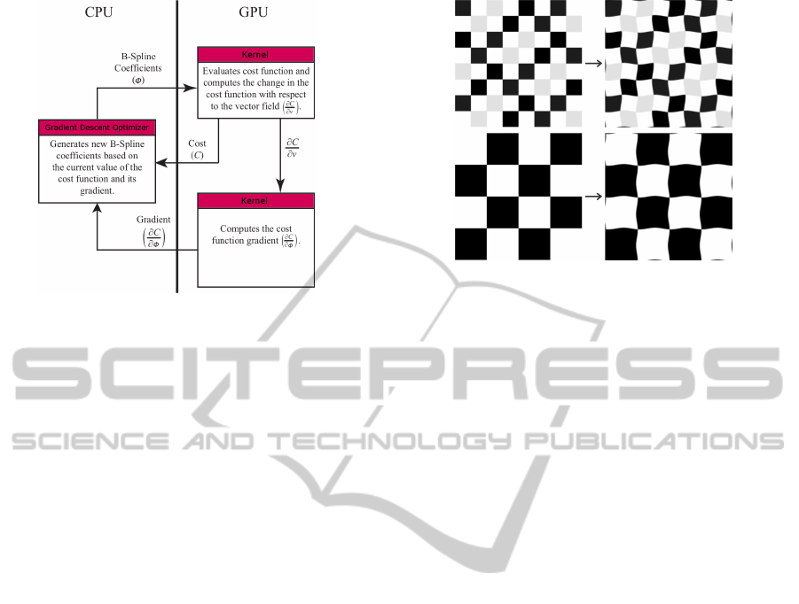
Figure 4: Framework organization.
transferred from GPU to the CPU for every iteration
of the image registration process. Transfers between
the CPU and GPU memories are the most costly in
terms of time, but Shackleford observed in his ex-
periments that the CPU-GPU communication over-
head demands roughly 0.14% if the total algorithm
execution time. This fact allows the conclusion that
the CPU-GPU transfers do not affect the overall algo-
rithm performance.
6 RESULTS
We have implemented two items: an image regis-
tration framework and an application that uses this
framework for finding the MCAP. Both have been
thoroughly evaluated and the results are described in
the following subsections.
6.1 Image Registration Evaluation
Given that the method for extracting the corpus callo-
sum area relies heavily on deformable registration, the
quality of the registration directly affects the accuracy
of the area measurement. Several experiments have
been conducted in order to evaluate the deformable
registration that was implemented. Synthetic data has
been used to demonstrate the effectiveness and perfor-
mance of the registration framework, but our frame-
work has also been evaluated with medical data.
To evaluate the effectiveness and performance of
the registration framework, ground truth experiments
have been conducted. The precision and error intro-
duced by the algorithm that has to be evaluated, can
be assessed by comparing the results with the ground
truth. In this case, a synthetic image is deformed
using a known control point configuration. This de-
Figure 5: Conducted experiment.
formed image will serve as the reference image, while
the original, undeformed image will act as the tem-
plate image. The quality of the registration can be
measured by comparing the displacement field ob-
tained by the registration framework with the ground
truth displacement field computed from the known
control point configuration.
For the experiments, two synthetic images where
used as shown on the left side in Figure 5. Both
images have a checkerboard pattern and are of size
256 × 256, inspired by the experiments conducted by
Schwarz (Schwarz, 2007). For both images, a sepa-
rate control point configuration was created that were
sinusoidal in both x- and y-direction and with a fixed
control point spacing of 15 pixels. Using these con-
trol point configurations, the displacement fields were
calculated for each original image together with the
resulting warped images as shown on the right side of
Figure 5. Next, the registration framework is utilized
with various control point spacings ranging from 5 to
50 pixels with increments of 5.
We have conducted three experiments to evaluate
the accuracy of our registration framework. First, we
calculated the similarity of the images (using SSD)
after the registration process (Figure 6). The next
experiment calculated the Root Mean Square Error
(RMSE) between the ground truth displacement field
and the displacement field obtained from the registra-
tion process (Figure 7). Last, we calculated the mag-
nitude of difference (Figure 8). Each of these experi-
ments individually validated the accuracy of our reg-
istration framework, as they show that a control point
spacing of 15−20 pixels best recovers the applied de-
formation.
For this paper, three versions of the image reg-
istration implementation were written: a na
¨
ıve CPU
and GPU implementation and an optimized GPU ver-
sion. All three implementations will generate the
same result, but will perform the registration at dif-
VISAPP2015-InternationalConferenceonComputerVisionTheoryandApplications
146
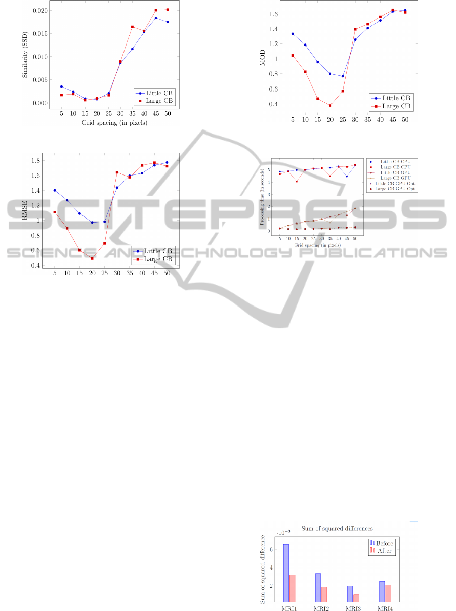
Figure 6: Similarity after registration.
Figure 7: RMSE of the generated displacement field and the
ground truth.
ferent speeds. Figure 9 shows the impact of differ-
ent control point spacings on the three implemented
versions. Both the GPU and CPU versions of the
na
¨
ıve implementation are susceptible to grid spacing,
because a coarse grid spacing means bigger tiles to
compute and a lot of redundant ∂C
sim
/∂
−→
v loads. The
performed experiments showed that when comparing
the GPU and CPU version of the na
¨
ıve implementa-
tion, for a grid spacing of 5 pixels, the GPU version
performed about 21 times faster than the CPU. When
reaching a grid spacing of 50 pixels, it only performed
three times faster than the CPU version.
The optimized GPU version, however, is rather
agnostic to grid spacing. At a grid spacing of 10 pix-
els, the optimized version performed about 24 to 40
times faster than the na
¨
ıve CPU version. When using
a grid spacing of 50 pixels, the optimized version cal-
culated its results about 20 times faster than its na
¨
ıve
CPU counterpart. Since the image registration frame-
work is an essential part in finding the MCAP, it is
paramount that this part was properly optimized.
The deformable registration framework has also
been evaluated using medical data. To assess the qual-
ity of the registration, two measurements were used,
namely the sum of squared differences (SSD) mea-
surement and the correlation coefficient (CC) mea-
surement, as shown by Figures 10 and 11 respec-
Figure 8: Magnitude of Difference of generated displace-
ment field and ground truth.
Figure 9: Processing time of registration using CPU, GPU
and the optimized GPU versions.
tively. The results show that the resulting warped
images significantly resemble their fixed image coun-
terparts. We have used three MRI data sets retrieved
from the Open Access Series of Imaging Studies (OA-
SIS) project as well as an MRI volume obtained from
icoMetrix. The OASIS project is aimed at making
MRI data sets of the brain available to the scientific
community. The volume of icoMetrix has a size of
79 × 95 × 68 voxels, while the three volumes from
OASIS have a size of 128 × 256 × 256 voxels. How-
ever, the three volumes from OASIS are anisotropic
in nature. Each of the volumes have been resampled
so that they are isotropic, which results in a volume
of size 160 × 256 × 256. For each of these volumes,
we extracted a plane that roughly resembles the mid-
sagittal plane that would serve as the fixed image.
Next, we also extracted from each volume a plane
that has been rotated over several degrees from the
central pixel of each volume’s extracted midsagittal
plane. The reason why we chose these planes is that
Figure 10: SSD between the fixed image and the warped
moving image before and after the registration process.
ComputingCorpusCallosumasBiomarkerforDegenerativeDisorders
147
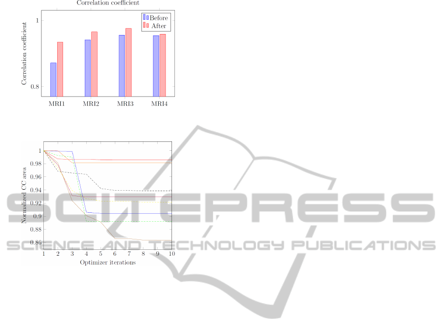
Figure 11: CC between the fixed image and the warped
moving image before and after the registration process.
Figure 12: Graph of normalized CC areas of 8 MRI vol-
umes.
this is exactly what the implemented application will
do when searching for the MCAP.
6.2 MCAP Extraction Evaluation
Figure 12 shows a graph of normalized corpus callo-
sum areas for 8 MRI volumes in function of the opti-
mizer iterations. Seven of these MRI volumes came
from the OASIS project and the other one came from
icoMetrix. The results for each volume have been
normalized (i.e. starting at 1) with the rotation param-
eters and the translation parameter set to zero. The re-
sults show a distinct decrease and convergence of the
corpus callosum area for all examined volumes.
For the examined volumes, we register a percent-
age drop ranged from a minimum of 0.01%, a max-
imum of 13.6889% with a mean decrease in area of
6.6094% and a median decrease of 7.5012%. As
stated by Ishaq (Ishaq, 2008) and longitudinal study
performed by Juha (Juha et al., 2007), the minimiza-
tion in corpus callosum area is potentially significant,
given that approximately 33% of the reduction in cor-
pus callosum area can be explained by atrophy.
7 CONCLUSIONS
The developed framework can automatically extract
the MCAP and simultaneously segment the corpus
callosum. This method, introduced by Ishaq, can aid
longitudinal studies. The method used, treats the cor-
pus callosum area as a function of the plane extrac-
tion parameters and it uses deformable registration to
generate a displacement field that can be used for the
calculation of the corpus callosum area. The gathered
results show a clear decrease and convergence to the
plane with minimal corpus callosum area.
The obtained results cannot be compared to other,
existing methods, because none of the existing meth-
ods try to achieve the same objective, which is the
identification of minimal corpus callosum area and
therefore, such a comparison would not be meaning-
ful. As stated by Ishaq, this work can benefit future
studies on longitudinal analysis of the change in cor-
pus callosum area with the progression of different
neurological diseases.
Deformable registration is a crucial part in find-
ing the MCAP. The algorithm for deformable regis-
tration has been described in detail. Free-form defor-
mation has been used, which allows to model flexi-
ble deformations by means of a limited grid of con-
trol points, instead of manipulating each pixel indi-
vidually as is done in deformable registration meth-
ods based on dense deformation fields. A regulariza-
tion term is also used that will penalize deformations
that are implausible.
Finding an MCAP requires multiple image regis-
tration iterations. Therefore, the registration frame-
work has been optimized using CUDA. The intro-
duced algorithms, optimizations and data structures
reduce the complexity of the B-spline registration
process. Highly parallel and scalable designs for
computing both the sum of squared differences sim-
ilarity measure and its derivative with respect to the
B-spline parameterization were implemented. The
speed and robustness of the image registration pro-
cess were determined using both synthetic and medi-
cal data. The acceleration of the GPU process ranges
from 24 to 40 times faster than the na
¨
ıve CPU imple-
mentation, depending on the grid spacing used for the
control points.
ACKNOWLEDGEMENTS
This research has been made possible thanks to the
collaboration with icoMetrix in Belgium.
VISAPP2015-InternationalConferenceonComputerVisionTheoryandApplications
148

REFERENCES
Aylward, S., Jomier, J., Barre, S., Davis, B., and Ibanez, L.
(2007). Optimizing ITK’s Registration Methods for
Multi-processor, Shared-memory Systems. MICCAI
Workshop on Open Source and Open Data.
Barr, A. (1984). Global and Local Deformations of
Solid Primitives. SIGGRAPH Computer Graphics,
18(3):21–30.
Bookstein, F. and Green, D. (1993). A feature space for
derivatives of deformation. Information Processing
in Medical Imaging - Lecture Notes in Computer Sci-
ence, 687:1–16.
Christensen, G., Rabbitt, R., and Miller, M. (1996). De-
formable templates using large deformation kine-
matics. IEEE Transactions on Image Processing,
5(10):1435–1447.
Compston, A. and Coles, A. (2008). Multiple Sclerosis. The
Lancet, 372(9648):1502–1517.
Davatzikos, C., Vaillant, M., Resnick, S., Prince, J.,
Letovsky, S., and Bryan, R. (1996). A Computerized
Approach for Morphological Analysis of the Corpus
Callosum. Journal of Computer Assisted Tomogra-
phy, 20(1):88–97.
Duning, T. and Kloska, S. (2005). Dehydration con-
founds the assessment of brain atrophy. Neurology,
64(3):548–550.
Hill, D., Batchelor, P., Holden, M., and Hawkes, D. (2001).
Medical Image Registration. Physics in Medicine and
Biology, 46(3):R1–R45.
Hubel, D. (1995). Eye, brain and vision. WH Freeman.
Ishaq, O. (2008). Algorithms for Image Analysis of Corpus
Callosum Degeneration for Multiple Sclerosis. Mas-
ter’s thesis, Simon Fraser University.
Juha, M., Leszek, S., Sten, F., Jakob, B., Olof, F., and Maria,
K. (2007). Non-age-related Callosal Brain Atrophy in
Multiple Sclerosis: A 9-year Longitudinal MRI Study
Representing Four Decades of Disease Development.
Journal of Neurology, Neurosurgery, and Psychiatry,
78:375–380.
Metaxas, D. (1997). Physics-Based Deformable Models:
Applications to Computer Vision, Graphics and Med-
ical Imaging. Kluwer.
Rohde, G., Aldroubi, A., and Dawant, B. (2003). The adap-
tive bases algorithm for intensity-based nonrigid im-
age registration. IEEE Transactions on Medical Imag-
ing, 22(11):1470–1479.
Rueckert, D., Sonoda, L., Hayes, C., Hill, D., Leach, M.,
and Hawkes, D. (1999). Nonrigid Registration Us-
ing Free-Form Deformations: Application to Breast
MR Images. IEEE Transactions on Medical Imaging,
18(8).
Schoenberg, I. (1946). Contributions to the Problem of Ap-
proximation of Equidistant Data by Analytic Func-
tions. The Quarterly of Applied Mathematics, 4:45–
99.
Schwarz, L. (2007). Non-rigid Registration Using Free-
from Deformations. Master’s thesis, Technische Uni-
versit
¨
at M
¨
unchen.
Sederberg, T. and Parry, S. (1986). Free-form Deformation
of Solid Geometric Models. SIGGRAPH Computer
Graphics, 20(4):151–160.
Shackleford, J. (2011). High-Performance Image Registra-
tion Algorithms for Multi-Core Processors. PhD the-
sis, Drexel University.
Shackleford, J., Kandasamy, N., and Sharp, G. (2010). On
developing B-spline registration algorithms for multi-
core processors. Physics in Medicine and Biology,
55:6329–6351.
Sharp, G., Peroni, M., Li, R., Shackleford, J., and Kan-
dasamy, N. (2010). Evaluation of Plastimatch B-
Spline Registration on the EMPIRE10 Data Set. Med-
ical Image Analysis for the Clinic: A Grand Chal-
lenge, pages 99–108.
Simon, J. (2006). Brain Atrophy in Multiple Sclerosis:
What We Know and Would Like to Know. Multiple
Sclerosis, 12(6):679–687.
Simon, J., Simon, L., Campion, M., Rudick, R., Cookfair,
D., Herndon, R., Richert, J., Salazar, A., Fischer, J.,
Goodkin, D., Simonian, N., Lajaunie, M., Miller, D.,
Wende, K., Martens-Davidson, A., Kinkel, R., Mun-
schauer, F., and Brownscheidle, C. (2006). A Longi-
tudinal Study of Brain Atrophy in Relapsing Multiple
Sclerosis. Neurology, 12(6):679–687.
Szeliski, R. and Coughlan, J. (1997). Spline-Based Image
Registration. International Journal of Computer Vi-
sion, 22(3):199–218.
Thirion, J. (1998). Image matching as a diffusion process:
an analogy with Maxwell’s demons. Medical Imaging
Analysis, 2(3):243–260.
Thompson, P. and Toga, A. (1996). A surface-based
technique for warping three-dimensional images of
the brain. IEEE Transactions on Medical Imaging,
15(4):402–417.
Unser, M. (1999). Splines: A Perfect Fit for Signal and
Image Processing. IEEE Signal Processing Magazine,
16(6):22–38.
ComputingCorpusCallosumasBiomarkerforDegenerativeDisorders
149
