Fast and Accurate Reﬁnement Method for 3D Reconstruction from

Stereo Spherical Images

Marek Solony

, Evren Imre

, Viorela Ila

, Lukas Polok

, Hansung Kim

and Pavel Zemcik

Faculty of Information Technology, Brno University of Technology, Brno, Czech Republic

Centre for Vision, Speech and Signal Processing, University of Surrey, Guildford, U.K.

Keywords:

Spherical Images Registration, 3D Reconstruction, Graph Optimisation, SLAM.

Abstract:

Realistic 3D models of the environment are beneﬁcial in many ﬁelds, from natural or man-made structure

inspection and volumetric analysis, to movie-making, in particular, special effects integration to natural scenes.

Spherical cameras are becoming popular in environment modelling because they capture the full surrounding

scene visible from the camera location as a consistent seamless image at once. In this paper, we propose

a novel pipeline to obtain fast and accurate 3D reconstructions from spherical images. In order to have a

better estimation of the structure, the system integrates a joint camera pose and structure reﬁnement step.

This strategy proves to be much faster, yet equally accurate, when compared to the conventional method,

registration of a dense point cloud via iterative closest point (ICP). Both methods require an initial estimate for

successful convergence. The initial positions of the 3D points are obtained from stereo processing of pair of

spherical images with known baseline. The initial positions of the cameras are obtained from a robust wide-

baseline matching procedure. The performance and accuracy of the 3D reconstruction pipeline is analysed

through extensive tests on several indoor and outdoor datasets.

1 INTRODUCTION

Nowadays, there is a large interest in recreating the

3D environment from images coming either from still

or moving cameras, in stereo or monocular setups.

Well-known applications such as Photo Tourism can

reconstruct tourist places from thousands of internet

images; Google’s 3D maps application can recon-

struct entire cities from aerial and satellite images.

Due to the limited ﬁeld of view of the conven-

tional cameras a large number of images needs to

be acquired in order to reconstruct outdoor or indoor

scenes. In applications involving large scenes, an ac-

ceptable coverage with still images can be a problem

due to both, time consuming acquisition process as

well as large memory requirements. One solution to

this is to use spherical cameras which cover 360

◦

the space. Only few such images are needed to create

a dense reconstruction of a large scene.

In this paper, we introduce a novel spherical im-

age processing pipeline to obtain fast and accurate 3D

reconstructions of a scene. The advantage of this sys-

tem is that it can recreate relatively large outdoor or

indoor scenes from only a handful of spherical im-

ages. In order to obtain a dense 3D reconstruction,

stereo pairs of spherical images are considered. Ac-

quiring stereo pairs is in general a simple task, since

most of the spherical imaging systems are placed on a

tripod which allows an exact adjustment of the height

of the camera, without introducing any rotations.

The processing pipeline has two parts; a) an ini-

tialisation step and b) a structure and camera pose

reﬁnement step. The initial positions of the 3D

points are obtained from a stereo processing frame-

work which produces an accurate disparity map from

stereo spherical image pairs with known baseline. To

obtain accurate depth from stereo pairs, dense dis-

parity maps are estimated using a multi-resolution

partial differential equation (PDE) (Kim and Hilton,

2013) based stereo matching algorithm which accel-

erates the calculation for large images whilst keeping

smooth surface and sharp object boundaries. The ini-

tial positions of the cameras are obtained from a ro-

bust wide-baseline matching procedure. The wide-

baseline nature of the problem necessitates the use

of robust estimators, such as RANSAC. Our geom-

etry estimation pipeline is an implementation of the

guided matching algorithm of (Hartley and Zisser-

man, 2003). It iterates over successive stages of

matching and RANSAC-based geometry estimation.

575

Solony M., Imre E., Ila V., Polok L., Kim H. and Zemcik P..

Fast and Accurate Reﬁnement Method for 3D Reconstruction from Stereo Spherical Images.

DOI: 10.5220/0005310805750583

In Proceedings of the 10th International Conference on Computer Vision Theory and Applications (VISAPP-2015), pages 575-583

ISBN: 978-989-758-091-8

 2015 SCITEPRESS (Science and Technology Publications, Lda.)

The initialisation is further used to either register

consecutive dense point clouds using Iterative Closest

Point (ICP) (Kim and Hilton, 2013) algorithms or to

perform joint pose and structure reﬁnement. The ICP

algorithm is widely used for geometric registration of

three dimensional point clouds when an initial esti-

mate of the relative pose is known (Besl and McKay,

1992; Rusinkiewicz and Levoy, 2001). ICP simply

ﬁnds a 3D rigid transformation matrix to minimize

the distance of the closest points between two point

clouds. It suffers from local minimum problem if the

initialisation is not close enough to the true solution.

On the other hand, the nonlinear structure reﬁne-

ment is based on joint optimisation of sparse 3D

points and camera poses. The problem is formulated

as a nonlinear optimisation on graphs (Dellaert and

Kaess, 2006; K

ummerle et al., 2011), where the nodes

are the 3D points and the 3D camera poses and the

edges are the relative point-camera transformations

(see section 4). The optimisation problem ﬁnds the

best cameras-points conﬁguration, given the impre-

cise relative positions of the 3D points obtained from

the initialisation step. Section 5 analyses the time and

performance of both approaches, the ICP based regis-

tration and the proposed reﬁnement method.

2 RELATED WORK

Building a representation of the environment from

noisy sensorial data is a central problem in com-

puter vision and robotics. Problems in computer

vision include bundle adjustment (BA) (Agarwal

et al., 2009) and structure from motion (SFM) (Beall

et al., 2010). Simultaneous localization and map-

ping (SLAM) (Dellaert and Kaess, 2006; Kaess et al.,

2008; K

ummerle et al., 2011) is a similar problem in

robotics. Those are mathematically equivalent tech-

niques, with a slight difference in the types of con-

straints: while BA minimizes the reprojection error,

SLAM minimizes the residual directly in the repre-

sentation space. The key to developing fast methods

in this direction is the interpretation of the problem

in terms of graphical models. Understanding the ex-

isting graphical model inference algorithms and their

connection to matrix factorization methods from lin-

ear algebra allowed computationally efﬁcient solu-

tions (Dellaert and Kaess, 2006; Snavely et al., 2006;

ummerle et al., 2011; Polok et al., 2013a).

For the particular problem of 3D reconstruction

from stereo spherical images, minimizing the repro-

jection error in the image space may not be the

best approach. This is due to the fact that in the

spherical images, the reprojection error, which is the

distance between measured and estimated 2D point,

varies with the latitude of unwrapped spherical image.

Therefore, a more correct approach is to optimize di-

rectly in the representation space applying SLAM op-

timisation methods.

While the BA approaches use sets of still im-

ages from unrelated viewpoints and possibly different

cameras with different parameters, SfM uses video

sequences from a moving camera to reconstruct a

3D model of the observed environment. The dis-

advantage of both, is the great number of images

needed to cover large areas. A common way to cap-

ture the full 3D space is to use a catadioptric om-

nidirectional camera using a mirror combined with

a charge-coupled device (CCD) (Hong et al., 1991;

Nayar, 1997). Lhuillier proposed a scene reconstruc-

tion system using omnidirectional images (Lhuillier,

2008). However, catadioptric omnidirectional cam-

eras have a large number of systematic parameters to

calibrate. Another problem is the limited resolution

because they use only one CCD to capture the full

3D space. Feldman and Weinshall used a Cross Slits

(X-Slits) projection with a rotating ﬁsheye camera to

acquire high quality spherical images while reduc-

ing the number of camera parameters and to generate

distortion-free image-based rendering (Feldman and

Weinshall, 2005). Kim and Hilton used this spherical

imaging to acquire multiple pairs of high-resolution

stereo spherical images and reconstructed full 3D ge-

ometry of the scene (Kim and Hilton, 2013). Note that

using omnidirectional or wide ﬁeld of view cameras

decreases the ratio of the number of cameras to the

number of observed points, as opposed to the tradi-

tional cameras. As will be shown later, this is beneﬁ-

cial for efﬁcient optimisation, as the resulting system

matrix sparsity patterns are favourable for solving us-

ing Schur complement (Zhang, 2005).

3 SPHERICAL IMAGE

PROCESSING

Using stereo spherical images from one or multiple

view-points is an easy and feasible way to create 3D

models of large environments. To obtain a 3D struc-

ture from stereo spherical images, image processing

algorithms are applied followed by a structure reﬁn-

ing procedure. This section describes an image pro-

cessing pipeline which inputs spherical images and

outputs an initial estimation for the reﬁning step.

3.1 Spherical Images

A spherical image is captured by a vertical line-scan

VISAPP2015-InternationalConferenceonComputerVisionTheoryandApplications

576

camera with wide-angle lens rotating around the cen-

tre of projection. The ﬁnal image is created by joining

scans into a single image so it covers 360

◦

in horizon-

tal and ≈ 180

◦

in vertical ﬁeld of view. This process is

equivalent to projecting the scene around the camera

onto a unit sphere and unwrapping it into a plane.

Compared to the images from conventional cam-

eras, the spherical images contain more information

in a single image and therefore more features can

be extracted for the purpose of estimating the rela-

tions between cameras. The main disadvantage of

the spherical images is the distortion introduced by

the wide-angle lenses and the rotating camera sen-

sor. The same parts of the scene viewed from dif-

ferent positions of the camera, appear very different

(see Fig. 1 b)). This can cause problems when ex-

tracting and matching features, especially when the

images are captured with wide baseline.

3.2 Stereo Processing

A stereo image pair with vertical disparity can be

obtained by placing the spherical camera at differ-

ent heights. Assuming that the images are precisely

aligned, the stereo-matching problem can be reduced

to a one-dimensional search on a line. The disparity

map is computed by processing all the columns of the

stereo image pair, and therefore the 3D position of any

valid 2D point can be obtained through a simple tri-

angulation. If pixels on the column are mapped to the

[0,π] range in the spherical coordinate, the disparity

d between projection points p

) and p

)

of a 3D point P to the stereo image pair I

and I

deﬁned as the difference of the vertical angles of the

projected points θ

and θ

as in:

d(p

) = θ

− θ

. (1)

The depth D

(the distance between the top camera

and the 3D point P) can be calculated by triangulation

as in Eq. (2) using the baseline distance B in addition

to the angular disparity.

) = B/



sinθ

tan(θ

+ d(p

))

− cosθ



(2)

A number of studies have been reported on the dispar-

ity estimation problem since the 1970 (Scharstein and

Szeliski, 2002). Any disparity estimation algorithm

can be used for our system as long as it produces accu-

rate and dense disparity. Most disparity estimation al-

gorithms solve the correspondence problem on a dis-

crete domain such as integer or half-pixel levels which

are not sufﬁcient to recover a smooth surface. Espe-

cially spherical stereo image pairs can show more se-

rious artefacts in the reconstruction because they have

a serious radial distortion. A variational approach

which theoretically works on a continuous domain

can be a solution for accurate ﬂoating-point disparity

estimation. We use a PDE-based variational dispar-

ity estimation method to generate accurate disparity

ﬁelds with sharp depth discontinuities for surface re-

construction (Kim and Hilton, 2013).

3.3 Feature and Descriptors Extraction

The estimation of the relative pose between two

spherical cameras requires a set of reliable 3D point

correspondences. 3D features from each camera are

selected by detecting 2D SIFT features on the spher-

ical images, and computing the associated 3D coor-

dinates, by projecting them to the 3D space via the

computed depth map (section 3.2). Each 3D point is

characterised by the 2D SIFT descriptor of its cor-

responding 2D feature on the spherical image (

Imre

et al., 2010). This process generates a sparse 3D point

cloud for each camera and its corresponding descrip-

tor as input to the initial pose estimation stage.

3.4 Computation of the Initial Pose

Estimate

The computation of the initial pose estimate follows

the conventional guided matching pipeline, which in-

volves alternating stages of feature matching and ge-

ometry estimation (Hartley and Zisserman, 2003).

The pipeline requires two sets of 3D features as in-

put. It returns H

, the initial 3D pose estimate, and I ,

the 3D correspondences supporting H

The feature matching stage seeks for nearest

neighbours, by comparing the associated SIFT de-

scriptors (Lowe, 2004). However, the pipeline often

operates under wide-baseline conditions, which sig-

niﬁcantly reduces the number of viable matchings.

Therefore, the implementation resorts to a compro-

mise between ambiguity and quantity, and considers

the 7 nearest neighbours, instead of the best. Each

candidate is veriﬁed for reciprocity, i.e. whether the

points are in each other’s neighbourhoods. Exces-

sively ambiguous matches are rejected by truncating

the neighbourhoods so that, the ratio of the similarity

scores for the worst candidate within the neighbour-

hood and the best candidate without is above a thresh-

old. The remaining correspondences are ranked by

the MR-Rayleigh metric (V.Fragoso and Turk, 2013).

The wide-baseline nature of the problem and the

multiple-element neighbourhoods imply a correspon-

dence set with many outliers. In geometry estima-

tion, such problems are typically solved by the help of

FastandAccurateRefinementMethodfor3DReconstructionfromStereoSphericalImages

577

RANSAC (Fischler and Bolles, 1981). RANSAC ap-

plies a hypothesise-and-test framework on small, ran-

domly selected sets of correspondences, in its search

for a set without any outliers.

For pose estimation, we generate the hypothe-

ses via (Horn, 1987), which requires 3-element sam-

ples. Our RANSAC implementation minimises the

symmetric transfer error (Hartley and Zisserman,

2003). It makes use of MSAC (Torr and Zisser-

man, 2000), LO-RANSAC (Chum et al., 2003), bi-

ased sampling (Chum and Matas, 2005) and Wald-

SAC (Chum and Matas, 2008). MSAC and LO-

RANSAC improves the estimate accuracy, through

better hypothesis assessment, and a local optimisa-

tion step to improve promising hypotheses, respec-

tively. Biased sampling steers the hypothesis gener-

ation towards samples with a better likelihood of be-

ing inliers (as indicated by the correspondence rank-

ing). WaldSAC allows the rejection of poor hypothe-

ses without testing the entire correspondence set, and

therefore, provides signiﬁcant computational savings.

RANSAC terminates when it is conﬁdent that a better

solution is unlikely (Chum and Matas, 2008), return-

ing H

and I .

3.5 Iterative Closest Point for 3D Point

Cloud Registration

One way to obtain a 3D dense reconstruction from

spherical stereo images is to use the camera pose esti-

mation from the previous step as an initialisation of a

dense 3D point-cloud registration. The 3D points are

obtained from the depth map computed as in 3.2 and

they are registered using ICP algorithm.

The ICP algorithm has been widely adopted to

align two given point sets (Besl and McKay, 1992;

Rusinkiewicz and Levoy, 2001). It ﬁnds a rigid

3D transformation (rotation R and translation t) be-

tween two overlapping clouds of points by iteratively

minimising squared-error of registration between the

nearest points from one set to the other:

(R,t) =

∑

i, j

− (Rd

+t)k

(3)

where N

and N

are the number of points in the

model set m and reference set d, respectively, and w

i, j

are the weights for a point match.

In each ICP iteration, the rigid 3D transforma-

tion can be efﬁciently calculated by either singular

value decomposition (SVD) (Arun et al., 1987) or

the closed-form solution (Horn, 1987). The closed-

form solution solves the least-squares problem for

three or more points using a unit quaternion to repre-

sent rotation or using manipulation matrices and their

eigenvalues-eigenvector decomposition.

When applied to dense point cloud registration,

the ICP algorithm can become very slow. Therefore,

in this work, we propose a method which reﬁnes a

sparse structure and the camera poses, and creates

the dense reconstruction by referring the dense point-

clouds to the accurately estimated camera positions.

4 JOINT POSE AND STRUCTURE

REFINEMENT

In order to obtain an accurate 3D structure, the pro-

posed pipeline performs a joint optimisation of the

initial camera poses and the corresponding sparse

point clouds. The problem is formulated as a nonlin-

ear optimisation on graphs, where the vertices are the

absolute points and camera poses and the edges are

relative point-camera transformations obtained from

the depth map. Said differently, the vertices are the

variables to be estimated and the edges are the mea-

sured constraints. To obtain an optimal conﬁguration

of the graph, we perform a maximum likelihood esti-

mation (MLE).

Under the assumption of zero-mean Gaussian

measurement noise, the MLE has a nonlinear least

squares (NLS) solution. The goal is to obtain the

MLE of a set of variables θ = [θ

...θ

], containing

the 3D points in the environment p = [p

... p

] and

the camera poses c = [c

...c

], given the set of 3D

relative measurements, z = [z

...z

∗

= argmax

P(θ | z) = argmin

{

−log(P(θ | z)

}

(4)

This measurement can be modelled as a function

, p

) of the camera c

and the point p

with zero-

mean Gaussian noise with the covariance Σ

P(z

| c

, p

) ∝ exp



−

k z

− h(c

, p

) k



, (5)

Finding the MLE from (4) is done by solving the fol-

lowing nonlinear least squares problem:

∗

= argmin

(

∑

k=1



− h(c

, p

)



)

. (6)

Iterative methods such as Gauss-Newton (GN) or

Levenberg-Marquard (LM) are used to ﬁnd the solu-

tion of the NLS in (6). An iterative solver starts with

an initial point θ

and, at each step, computes a cor-

rection δ towards the solution. For small

, a Taylor

series expansion leads to linear approximations in the

neighbourhood of θ

e(θ

+ δ) ≈ e(θ

) + Jδ , (7)

VISAPP2015-InternationalConferenceonComputerVisionTheoryandApplications

578

where e = [e

,...,e

]

is the set of all nonlinear er-

rors between the estimated and the actual measure-

ment, e

, p

) = z

− h(c

, p

), with [c

, p

] ⊆ θ

and J is the Jacobian matrix which gathers the deriva-

tive of the components of e. Thus, at each iteration i,

a linear LS problem is solved:

∗

= argmin

A δ − b

, (8)

where the A = Σ

−>\2

J(θ

) is the system matrix,

b = e(θ

) the right hand side (r.h.s.) and δ = (θ − θ

)

the correction to be calculated (Dellaert and Kaess,

2006). The the minimum is attained where the ﬁrst

derivative cancels:

A δ = A

b or Λδ = η , (9)

with Λ = A

A, the square symmetric system matrix

and η = A

b, the right hand side. The solution to the

linear system can be obtained either by sparse ma-

trix factorization followed by backsubstitution or by

linear iterative methods. After computing δ, the new

linearisation point becomes θ

i+1

= θ

⊕ δ.

In our application the initial solution θ

can be rel-

atively far from the minimum, therefore LM is pre-

ferred over the GN methods. LM is based on ef-

ﬁcient damping strategies which allow convergence

even from poor initial solutions. For that, LM solves

a slightly modiﬁed variant of (9), which involves a

damping factor λ:

(Λ + λ

D)δ = η or Hδ = η , (10)

where

D can be either the identity matrix,

D = I, or

the diagonal of the matrix Λ,

D = diag(Λ).

Schur complement is employed to solve the lin-

earised problem in (10). For that, the system matrix

is split in four blocks, according to the camera and

points variables:



C U











(11)

This is a common practice in solving 3D reconstruc-

tion problems, where the camera poses are linked only

through the points. It results in diagonal C and P ma-

trices, which can be easily inverted. If P is invertible,

the Schur complement of the block P is C −UP

−1

and is used to solve for the camera poses ﬁrst. Points

are then obtained by solving the remaining system.

Performing matrix inversion and multiplication in

the Schur complement form brings reduction in com-

putational time, compared to performing Cholesky

factorisation of the whole system. To improve conver-

gence, after every iteration of the nonlinear solver, the

state of the cameras is ﬁxed and three iterations opti-

mising only the points are performed. This is based

on the observation, that while a single camera may

depend on a large number of points, a single point is

usually only observed from two or three cameras, and

as such the positions of the points are harder to esti-

mate precisely. The extra iterations allow the points

to settle before performing the following nonlinear

solver iterations. In our experiments, the extra iter-

ations reduce residual as efﬁciently as the full non-

linear iterations, only at much smaller computational

cost. A similar technique was described in (Jeong

et al., 2012).

The result of the estimation is an optimised con-

ﬁguration of the sparse 3D structure p and the camera

poses c. The dense structure is obtained by referring,

for each pixel, its 3D position from the depth map to

the optimised camera poses.

5 EVALUATIONS AND RESULTS

This section evaluates the automatic process of align-

ing multiple spherical cameras in the terms of accu-

racy and computation time.

5.1 Datasets

Multiple experiments were performed in order to

evaluate the performance of the proposed 3D recon-

struction from stereo spherical images using three

spherical image datasets; two outdoor datasets, cover-

ing large area: Cathedral and CCSR, and one indoor

dataset with measured ground truth: Studio. The im-

ages were acquired with a SpheroCam-HDR system,

which captures scan lines with turning ﬁsheye lenses,

synthesises them and provides a 50 Mpix latitude-

longitude image. For Cathedral and CCSR dataset,

the camera was placed in three different positions

around the scene and for Studio dataset, four posi-

tions have been used. Each capture was done at two

different heights to produce stereo image pairs.

The Cathedral dataset covers an area of about

2500 m

. In order to test how the system per-

forms in the case of large sensor displacements, the

cameras were placed at positions far apart (approx.

18 m in the Cathedral dataset). The CCSR dataset

has shorter sensor displacements, and covers an area

about 250 m

. Studio dataset was captured with the

purpose to evaluate the pipeline in a short sensor dis-

placement setting (approx. 1 m). All details about

datasets are included in Table 1.

5.2 Evaluation Modules

Several modules can be distinguished in the stereo im-

FastandAccurateRefinementMethodfor3DReconstructionfromStereoSphericalImages

579

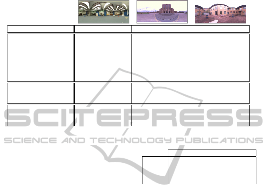
Table 1: Top: Dataset descriptions; Bottom: Time required to process image pairs.

Characteristics Studio Cathedral CCSR

Ground truth Measured GT ICP GT ICP GT

Stereo baseline [m] 0.2 0.6 0.2

Sensor displacement [m] 1.00/2.00/1.00 19.38/17.04 5.81/5.22

Cameras 4 3 3

Matches 754/340/997 546/488 2584/2150

Vertices 1715 681 2832

Edges 3653 1425 6048

Processing

Feat. & desc. extract [s] 8.15 7.02 6.32

Initial estimation [s] 6.99 11.41 25.65

Reﬁnement

ICP [s] 146.057 366.024 995.43

SLAM++[s] 0.120 0.091 0.134

age processing pipeline: depth map calculation, fea-

ture extraction, matching and initial pose and struc-

ture estimation and reﬁnement. The steps are illus-

trated in Figure 1. The stereo spherical image pro-

cessing pipeline and the graph optimisation for pose

and sparse structure reﬁnement were implemented in

C / C++. For the ICP registration a standard im-

plementation provided by the PCL library (Rusu and

Cousins, 2011) was used.

Iterative Closest Point (ICP)

Dense registration using ICP has been successfully

used in the literature for the 3D reconstruction from

spherical images (Kim and Hilton, 2013). There-

fore, ICP is used as a reference in the time and accu-

racy evaluations of the proposed reﬁnement method.

To calculate the initial estimate of the camera poses

and the 3D structure, the proposed image processing

pipeline is used. In the following text, we refer to this

simply as ICP.

Furthermore, we use dense ICP to deﬁne a ground

truth for testing the accuracy of our method in the

outdoor datasets where there are no manual measure-

ments available. For that manually matched sparse

features are used to calculate an initial estimate for

the ICP registration, and it will be further refers in the

paper as GT-ICP.

Joint Pose and Structure Reﬁnement

The joint pose and structure reﬁnement is based on

our open-source, nonlinear graph optimisation library,

called SLAM++ (Polok et al., 2013b). This is a very

Table 2: Depth map accuracy results: Differences between

GT and measurements in the depth map.

Sofa 1 Sofa 2 Table Carpet

P1 [cm] 1.8 1.2 0.2 0.3

P2 [cm] - - 0.7 0.8

P3 [cm] - - 7.8 0.1

P4 [cm] 1.7 3.2 1.3 0.3

efﬁcient implementation of nonlinear least squares

solvers, based on fast sparse block matrix manipula-

tion for solving the linearised problems. SLAM++

produces fast, but accurate estimations, which many

times outperform similar state-of-the-art implemen-

tations of graph optimisation systems. This perfor-

mance it is achieved due to the fact that the imple-

mentation exploits the block structure the problems

and offers very fast solutions to manipulate block ma-

trices and perform arithmetic operations. Edges and

vertices are deﬁned according to section 4 and the op-

timisation is performed on the manifold, therefore it

is correctly handling the derivatives of rotations and

translations. There are no simpliﬁcations or approxi-

mations involved in the optimisation process.

5.3 Time Evaluation

The disadvantage of applying ICP for image registra-

tion is its processing time. The approach proposed

in this paper offer much faster solutions in this direc-

tion. Table 1, bottom, shows that SLAM++ is, for all

datasets, almost three orders of magnitude faster than

the ICP algorithm. The good time performance stems

from the fact that it optimises for a sparse set of points

VISAPP2015-InternationalConferenceonComputerVisionTheoryandApplications

580

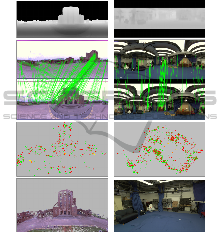
Cathedral Studio

Figure 1: Processing pipeline a) depth map b) inliers after matching with RANSAC algorithm (for better visibility only a

fraction of matches is shown for Studio dataset). Please note that the crossing lines in the left column are not outliers, the

image is spherical so the left part of the image continues on the right. c) initial (in red) vs. optimised (in green) poses and

sparse point cloud d) ﬁnal dense 3D reconstruction.

and from the actual implementation based on sparse

block solutions to non-linear least squares estimators.

By analysing the processing time of each step of

the pipeline in Table 1, we see that the time of opti-

mising the camera poses is now very small compared

to the other processing times in the pipeline, while

using ICP, the registration time would have been the

predominant time and would have constituted a bot-

tleneck in large applications.

5.4 Accuracy Evaluation

In our pipeline we can identify two sources of er-

rors that can affect the ﬁnal reconstruction, a) the

FastandAccurateRefinementMethodfor3DReconstructionfromStereoSphericalImages

581

Table 3: Accuracy results: Top: Structure Error. Bottom: Camera pose error evaluated separately for the rotation and

translation.

Criteria Method

Studio Cathedral CCSR

S1-S2 S2-S3 S3-S4 S1-S2 S2-S3 S1-S2 S2-S3

Pose Error

SLAM++ [cm] 0.46 0.79 1.12 70.87 37.14 37.49 11.93

ICP [cm] 1.07 3.61 5.08 67.83 74.05 26.11 14.99

SALM++ [degree] 1.14 0.57 0.89 5.48 3.91 0.81 1.66

ICP [degree] 5.03 0.81 1.38 4.85 4.83 0.52 2.71

Structure Error

SALM++ [cm] 1.61 112.02 48.89

ICP [cm] 3.54 176.56 39.47

error of the depth map and b) the camera pose es-

timation error. To analyse the accuracy of the pro-

posed technique, ground truth data were measured for

all three datasets. Smaller sensor displacement and

ﬂat ground surface of the Studio dataset allowed for

precise positioning of spherical cameras, and manual

measurements of distances from the spherical cam-

era positions to several objects in the scene as well

as distances between camera poses. For the outdoor

datasets, Cathedral and CCSR, the ground truth data

was generated by manually matching sparse features

to create an initialisation for the dense ICP (GT-ICP).

The error of the depth map was evaluated for

the Studio dataset by comparing the calculated depth

from the dense stereo processing with the measured

ground truth. In this dataset, the cameras were placed

in four different position with a know distance in be-

tween, and distance to objects in the scene (two dis-

tances to the sofa, one to the carpet, and one to the

desk) were measured. Table 2 shows the errors in

cm between the manually measured and the estimated

3D positions. The depth map error is, in average, of

1.6 cm for the Studio dataset. We can say that is a

very good depth calculation from stereo spherical im-

ages for indoor scenes, nevertheless, we should ex-

pect larger errors in the outdoor scenes.

In order to evaluate the joint camera and struc-

ture estimation, two types of errors are evaluated, a)

camera pose estimation error and b) structure error.

To compute the pose estimation error, the transfor-

mations between the GT-ICP and the estimated poses

are calculated. The errors in translation and rotation

are reported separately, by computing the norm of the

translation and the angle of rotation, respectively. For

each dataset, pair-wise spherical camera registrations

are evaluated. The structure error is computed in Stu-

dio dataset as average error of distances to known ob-

jects in scene and in the case of Cathedral and CCSR

datasets the structure error is given by the average eu-

clidean distance between two dense point clouds - one

from GT-ICP and second from optimized solution.

Table 3 conﬁrms our expectations that both, ICP

and SLAM++ have similar accuracy, and that larger

errors in pose estimation correlate with errors in struc-

ture estimation. Note that for longer baselines, the

SLAM++ copes better with the errors in the initial es-

timation compared to ICP which requires very good

initialisations. This is due to the fact that unlike

ICP which relies only on matches between consecu-

tive spherical cameras for each registration, SLAM++

also considers matches over multiple spherical im-

ages.

6 CONCLUSIONS AND FUTURE

WORK

The contribution of this paper is the formulation of

the 3D reconstruction from spherical images in terms

of sparse SLAM and based on that, obtaining a much

faster, yet accurate solution than the existing meth-

ods based on dense ICP. The efﬁciency comes from

both, the algorithm and the highly efﬁcient sparse

block matrix implementation of the nonlinear solver

used in jointly reﬁning the structure and the camera

poses. An initial estimate of the 3D points and the

camera positions is obtained from stereo processing

of pair of spherical images with known baseline and

a robust wide-baseline matching procedure. After the

initialisation, the structure can be reﬁned either via

dense point cloud registration or joint camera pose

and sparse structure optimisation. The later offers a

much faster alternative to ICP while maintaining sim-

ilar accuracy. The speed of the proposed approach

was at least three orders of magnitude faster than ICP

on all the datasets. It also offers a more robust es-

timation capable of exploiting relationships between

multiple spherical images and reﬁnes the solution ac-

cording to those constraints, whereas the ICP algo-

rithm works only pair-wise. The same approach can

be also easily applied in reconstruction from RGB-D

cameras where the 2D image features and the corre-

sponding 3D points can be reﬁned similarly to those

from stereo spherical images.

VISAPP2015-InternationalConferenceonComputerVisionTheoryandApplications

582

The proposed approach performs the optimisation

on sparse structure and then transforms the dense

point clouds by the calculated camera transforma-

tions. This yields a valid result, however, it may be

possible to obtain a more precise dense point cloud

alignment. Since the relation between the sparse

points and points from the dense point cloud are

known, it is possible to calculate a rigid transfor-

mation that aligns the dense point cloud to the cor-

responding sparse points (e.g. using (Horn, 1987)).

Further work will expand in this direction.

ACKNOWLEDGEMENTS

The research leading to these results has received

funding from the European Union, 7

Frame-

work Programme grants 316564-IMPART and the

IT4Innovations Centre of Excellence, grant n.

CZ.1.05/1.1.00/02.0070, supported by RDIOP funded

by Structural Funds of the EU and the state budget of

the Czech Republic.

REFERENCES

Agarwal, S., Snavely, N., Simon, I., Seitz, S. M., and

Szeliski, R. (2009). Building rome in a day.

Arun, K., Huang, T., and Blostein, S. (1987). Least square

ﬁtting of two 3-d point sets. IEEE Trans. Pattern Anal-

ysis and Machine Intelligence, 9(5):698–700.

Beall, C., Lawrence, B., Ila, V., and Dellaert, F. (2010). 3D

Reconstruction of Underwater Structures.

Besl, P. and McKay, N. (1992). A method for registration

of 3-D shapes. 14(2).

Chum, O. and Matas, J. (2005). Matching with PROSAC -

Progressive Sample Consensus. In Proc. CVPR, pages

220–226.

Chum, O. and Matas, J. (2008). Optimal Randomized

RANSAC. IEEE Transactions on Pattern Analysis

and Machine Intelligence, 30(8):1472–1482.

Chum, O., Matas, J., and Kittler, J. (2003). Locally Opti-

mized RANSAC. In Lecture Notes in Computer Sci-

ence, volume 2781, pages 236–243. Springer.

Dellaert, F. and Kaess, M. (2006). Square Root SAM: Si-

multaneous localization and mapping via square root

information smoothing. 25(12):1181–1203.

Feldman, D. and Weinshall, D. (2005). Realtime ibr with

omnidirectional crossed-slits projection. In Proc.

ICCV, pages 839–845.

Fischler, M. A. and Bolles, R. C. (1981). Random sample

consensus: A Paradigm for Model Fitting with Appli-

cations to Image Analysis and Automated Cartogra-

phy. Communications of the ACM, 24(6):381–395.

Hartley, R. and Zisserman, A. (2003). Multiple View Geom-

etry in Computer Vision. 2nd edition.

Hong, J., Tan, X., Pinette, B., Weiss, R., and E.M., R.

(1991). Image-based homing. In Proc. ICRA, pages

620–625.

Horn, B. K. P. (1987). Closed-form Solution of Absolute

Orientation Using Unit Quaternions. Journal of the

Optical Society of America A, 4(4):629–642.

Imre, E., Guillemaut, J.-Y., and Hilton, A. (2010). Moving

Camera Registration for Multiple Camera Setups in

Dynamic Scenes. In Proc. BMVC, pages 1–12.

Jeong, Y., Nister, D., Steedly, D., Szeliski, R., and

Kweon, I.-S. (2012). Pushing the envelope of mod-

ern methods for bundle adjustment. Pattern Analy-

sis and Machine Intelligence, IEEE Transactions on,

34(8):1605–1617.

Kaess, M., Ranganathan, A., and Dellaert, F. (2008). iSAM:

Incremental smoothing and mapping. 24(6):1365–

1378.

Kim, H. and Hilton, A. (2013). 3d scene reconstruction

from multiple spherical stereo pairs. International

Journal of Computer Vision, 104(1):94–116.

ummerle, R., Grisetti, G., Strasdat, H., Konolige, K., and

Burgard, W. (2011). g2o: A general framework for

graph optimization. In Proc. of the IEEE Int. Conf. on

Robotics and Automation (ICRA), Shanghai, China.

Lhuillier, M. (2008). Automatic scene structure and camera

motion using a catadioptric system. Computer Vision

and Image Understanding, 109(2):186–203.

Lowe, D. (2004). Distinctive image features from scale-

invariant keypoints. 60(2):91–110.

Nayar, S. (1997). Catadioptric omnidirectional camera. In

Proc. CVPR, pages 482–488.

Polok, L., Ila, V., Solony, M., Smrz, P., and Zemcik, P.

(2013a). Incremental block cholesky factorization for

nonlinear least squares in robotics. In Proceedings of

the Robotics: Science and Systems 2013.

Polok, L., Solony, M., Ila, V., Zemcik, P., and Smrz, P.

(2013b). Efﬁcient implementation for block matrix

operations for nonlinear least squares problems in

robotic applications. In Proceedings of the IEEE In-

ternational Conference on Robotics and Automation.

IEEE.

Rusinkiewicz, S. and Levoy, M. (2001). Efﬁcient variants

of the icp algorithm.

Rusu, R. B. and Cousins, S. (2011). 3D is here: Point Cloud

Library (PCL). In Proc. ICRA.

Scharstein, D. and Szeliski, R. (2002). A taxonomy and

evaluation of dense two-frame stereo correspondence

algorithms. International Journal of Computer Vision,

47(1):7–42.

Snavely, N., Seitz, S. M., and Szeliski, R. (2006). Photo

tourism: exploring photo collections in 3d. ACM

transactions on graphics (TOG), 25(3):835–846.

Torr, P. H. S. and Zisserman, A. (2000). MLESAC: A New

Robust Estimator with Application to Estimating Im-

age Geometry. Computer Vision and Image Under-

standing, 78(1):138–156.

V.Fragoso and Turk, M. (2013). SWIGS: A Swift Guided

Sampling Method. In Proc. of IEEE Conf. on Com-

puter Vision and Pattern Recognition (CVPR), pages

2770–2777, Portland, Oregon.

Zhang, F. (2005). The Schur complement and its applica-

tions, volume 4. Springer.

FastandAccurateRefinementMethodfor3DReconstructionfromStereoSphericalImages

583