
Performance Assessment and Interpretation of Random Forests by
Three-dimensional Visualizations
Ronny H
¨
ansch and Olaf Hellwich
Computer Vision and Remote Sensing, Technische Universit
¨
at Berlin, Marchstr.23, MAR6-5, 10587 Berlin, Germany
Keywords:
Random Forest, Randomized trees, Binary decision trees, Visualization.
Abstract:
Ensemble learning techniques and in particular Random Forests have been one of the most successful machine
learning approaches of the last decade. Despite their success, there exist barely suitable visualizations of
Random Forests, which allow a fast and accurate understanding of how well they perform a certain task and
what leads to this performance. This paper proposes an exemplar-driven visualization illustrating the most
important key concepts of a Random Forest classifier, namely strength and correlation of the individual trees
as well as strength of the whole forest. A visual inspection of the results enables not only an easy performance
evaluation but also provides further insights why this performance was achieved and how parameters of the
underlying Random Forest should be changed in order to further improve the performance. Although the paper
focuses on Random Forests for classification tasks, the developed framework is by no means limited to that
and can be easily applied to other tree-based ensemble learning methods.
1 INTRODUCTION
Over the last years Ensemble Learning (EL) tech-
niques gained more and more importance. Instead
of trying to create a single, highly optimal learner,
EL methods create many sub-optimal (base-)learners
and combine their output. Depending on the type of
base-learner, whether they are trained independently
or not, and how their output is used to create the final
system answer (e.g. by selection or fusion), the indi-
vidual EL approaches have been given many names,
as for example mixture of experts, consensus aggrega-
tion, bagging, boosting, arcing - to name only a few of
them (see e.g. (H
¨
ansch, 2014) for more details). The
main advantages of EL techniques are: 1) Less effort
has to be spent on the training of the individual learn-
ers, because they are not meant to be highly accurate;
2) Diverse base-learners with different (and poten-
tially complementary) characteristics can be used and
combined; 3) By using specific fusion techniques it is
possible to find solutions that were not within the in-
dividual hypotheses space of the single base-learners.
Especially the usage of decision trees within the
EL framework has shown large success. The in-
trinsic properties of such trees (e.g. low bias with
high variance, fast induction and training, built-
in feature selection, easy randomization, etc.) are
in perfect accordance to the underlying principles
of EL and thus naturally exploited. Consequently,
many different variations have been introduced: Ran-
dom Forest (Breiman, 2001), Extremely Randomized
Trees (Geurts and Wehenkel, 2006), Rotation Trees
(Rodriguez et al., 2006), Projection-based Random
Forests (H
¨
ansch, 2014), and many more. The work of
(Breiman, 1996; Breiman, 2001) introduces Random
Forests (RFs) rather as a general concept, instead of
a specific algorithm. Nowadays, RFs are likely to be
the most commonly used variant of combining deci-
sion trees with EL. They can be used for classification
as well as regression tasks and have been applied to a
vast amount of different application scenarios.
Very few effort, however, has been carried out
in the direction of visualizing Random Forests. The
available methods are at least partly not RF-specific
and can be coarsely divided into four groups: 1) As
for other machine learning methods (e.g. multi-layer
perceptrons or convolutional neural networks) there
are of course abstract visualizations of the underly-
ing model (Figure 1(a)). However, these are rather
graphical models of the general algorithmic class in-
stead of a visualization of an individual instance of
this class. 2) As for any other classification or regres-
sion technique it is possible to evaluate result-driven
visualizations by providing a graphical interpretation
of the system answer. Figure 1(b) gives an example
of a classification result, that was created by a spe-
149
Hänsch R. and Hellwich O..
Performance Assessment and Interpretation of Random Forests by Three-dimensional Visualizations.
DOI: 10.5220/0005310901490156
In Proceedings of the 6th International Conference on Information Visualization Theory and Applications (IVAPP-2015), pages 149-156
ISBN: 978-989-758-088-8
Copyright
c
2015 SCITEPRESS (Science and Technology Publications, Lda.)
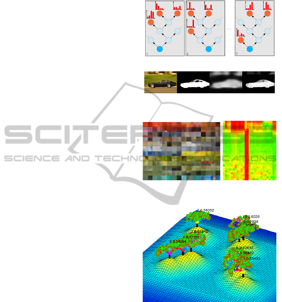
cific version of an RF in (H
¨
ansch, 2014). Since RFs
are able to provide a probabilistic output (although
not always used), they provide an intrinsic measure
of certainty of their solution, which can be exploited
in the corresponding visualization. 3) On the other
hand there are data-driven visualizations. In (Shot-
ton et al., 2008) RFs are used as a sophisticated clus-
tering technique which extracts specific image fea-
tures for the task of object recognition. Figure 1(c)
shows to which image pattern an individual tree re-
acts. This visualization gives a first coarse idea about
the features this method might be able to extract. Sim-
ilar data-driven visualizations are available for other
machine learning approaches as well, as for example
for convolutional neural networks (Zeiler and Fergus,
2014). 4) The last type, parameter-driven visual-
izations, are somewhat specific to Random Forests,
because they are one of the few methods that actually
provide some insight how the given task is solved and
do not just act as a black-box-system. The work of
(H
¨
ansch, 2014) discusses several of these properties
and how they can be visualized. One example is the
selection frequency of available features through the
forest like it is shown in Figure 1(d) for different fea-
tures (columns) per tree level (rows).
This work proposes a fifth type of visualization,
which is exemplar-driven. It combines the visualiza-
tion of the abstract model with parameter-driven vi-
sualizations and allows for deeper insights and faster
understanding of the trained forest. The basic idea of
the proposed method is given by the name “Random
Forest” itself: If this metaphorical name suits so well
as an algorithmical description, we will further extend
it to a full visualization of an actual forest as it is il-
lustrated in Figure 1(e).
2 RANDOM FORESTS
This section briefly describes the basic algorithm of
Random Forests. A detailed description of RFs is
beyond the scope of this work, but may be found in
the literature (e.g. (Breiman, 2001)). The following
discussion focuses on RFs for classification for the
sake of simplicity. The method proposed here is by
no means limited to that and can be applied to many
other types of tree-based EL.
A Random Forest consists of many binary
decision trees. These trees are inducted and trained
on a training set consisting of multidimensional data
points x and the desired system output (e.g. class
label) y. The work of (Breiman, 1996) proposed that
each tree has access only to a random part of the
(a) Model-driven: Abstract visualization of underlying
concepts (H
¨
ansch, 2014)
(b) Result-driven: Model-independent visualization of
(classification) results (From left to right: Image data, ref-
erence data, classification results of a two-stage framework
using ProB-RFs (H
¨
ansch, 2014))
(c) Data-driven: Visualization of
data in leaves of Semantic Texton
Forests (Shotton et al., 2008)
(d) Parameter-driven:
Visualization of feature
relevance of a ProB-RF
(H
¨
ansch, 2014)
(e) Exemplar-driven: Visualization of a specific RF
Figure 1: Different types of visualizing properties of a Ran-
dom Forest.
whole data set. This subset of the data enters the
tree at the root node. One of the data dimensions f
is randomly selected and a simple binary split is
performed. An example is given by Equation 1:
x
f
< θ (1)
where θ is a given threshold. All data points that
fulfill this test are propagated to the left child node,
IVAPP2015-InternationalConferenceonInformationVisualizationTheoryandApplications
150

all others to the right child node. The threshold θ can
be defined in many ways, for example by random
sampling, as median, or by criteria that optimize
the purity of the child nodes with respect to the
sample class distribution. This splitting is recursively
performed by all nodes, but always with different data
dimensions and thresholds. The recursive splitting
stops if a maximal tree height is reached or too few
data samples are available. In this case a terminal
node (leaf) is created, which simply estimates the
relative class-frequency P
t
(c|n
t
) of the data points,
that reached this leaf (node n
t
of tree t).
If the class label of a query data point x has to
be estimated, the query is propagated through all T
trees of the forest beginning at the root node. Its
way ends in exactly one leaf n
t
in each tree t. The
individual class probabilities P
t
(c|n
t
) of those leaves
are combined by a simple average (Eq. 2), which
provides the final estimate of the class’ a posteriori
distribution.
P(c|x) =
1
T
T
∑
t=1
P
t
(c|n
t
) (2)
Unlike many other machine learning approaches, RFs
not only provide measurements of the final perfor-
mance (e.g. classification accuracy) but also allow
insights into the actual properties of the inducted and
trained trees. Some of these measurements are sum-
marized in (H
¨
ansch, 2014). Here, only four of the
most important ones shall be mentioned, because they
play a special role within the visualization process de-
scribed in Section 3. The first one is the impurity of
the nodes of each tree. Each node has access to a spe-
cific subset of the whole dataset, namely the fraction
of samples that are propagated by its parent to this
node. During the training process these samples pro-
vide class labels which allow the computation of a lo-
cal estimate of the class distribution within this node.
There are several ways to measure the impurity of a
node, but the Gini impurity I as defined by Equation 3
is most commonly used.
I(n
t
) = 1 −
∑
c
P
t
(c|n
t
)
2
(3)
Since the final class decision of the forest is directly
based on the class estimates of the individual leaves,
the impurity of the leaves is of special importance.
The work of (Breiman, 2001) argues, that for EL
techniques in general and for RFs in particular, the
strength and the correlation of the individual
base-learners are two of the most important prop-
erties. Both characteristics are antagonistic to each
other: On the one hand, the stronger the individual
base-learners, the stronger is the whole forest. On
the other hand, the higher the correlation between
the base-learner, the less reasonable is it to combine
several of them. There is no point in creating many
trees, if they always provide the same estimate of the
class label (i.e. their correlation equals one). In other
words: It is important to create trees, which make
as few mistakes as possible, but when they do, then
it should be different mistakes. Only then the un-
derlying principles of EL can show their full potential.
In the case of RFs, the strength of the individ-
ual trees can be nicely estimated: Since each tree
is trained only on a subset of the whole dataset, the
remaining Z data points can be used to estimate a so
called Out-Of-Bag error, e.g. based on the 0-1-loss
E
01
as defined by Equation 4. This estimate gives a
good approximation of the generalization error of the
tree without the need of an additional holdout set.
E
01
=
1
Z
·
∑
x
(1 − δ(argmax(P
t
(c|n
t
)),y
x
)) (4)
The correlation Γ = [γ
(t
1
,t
2
)
] ∈ R
T ×T
of the trees is
measured as their agreement during classifying the
training data, i.e. γ
(t
1
,t
2
)
is the Pearson correlation co-
efficient of the classification results of the trees t
1
and
t
2
.
Last but not least, the strength of the whole for-
est is of interest. In contrast to the strength of a single
tree, it should be estimated on a holdout set, since the
forest as a whole has seen all samples of the training
dataset. Although RFs are not prone to overfitting, the
error estimate based on the training set will be biased
and should not be used as an approximation of the
generalization error. Instead, previously unseen sam-
ples of a test set are propagated through the forest to
determine their label. A confusion matrix E ∈ R
C×C
can be computed based on the estimated class labels
as well as the labels provided by the reference data.
This work uses the balanced accuracy BA defined by
Equation 5 as performance measure, since it is less
biased in case of imbalanced datasets.
BA =
1
C
C
∑
i=1
e
cc
Z
c
(5)
where C is the number of classes and Z
c
the number
of samples of class c and e
cc
is the c-th entry on the
main diagonal of E.
3 VISUALIZATION
This section explains how a given RF is visualized
based on its properties such as described in Section 2.
The first subsection focuses on the creation of a single
PerformanceAssessmentandInterpretationofRandomForestsbyThree-dimensionalVisualizations
151

tree, while Subsection 3.2 describes how the whole
forest is formed by multiple trees.
3.1 Tree Visualization
Each tree of an RF is a binary decision tree. There
are many approaches to visualize these simple types
of tree models. The method described in this paper
leads to a simple three-dimensional tree-structure,
that represents the underlying decision trees with
respect to its topology as well as basic properties
such as leaf impurity and selected features.
The root node of the tree is visualized as a ver-
tical line (orientation angles α = 90
◦
,β = 0
◦
). Length
and direction of the two child branches L and R are
based on the height h of these nodes and determined
by Equations 6-7.
(α,β)
L/R
h+1
= (α, β)
h
± (30
◦
,κ
1
· 45
◦
) (6)
l
L
h+1
= l
R
h+1
= l
h
· f (7)
where f = κ
2
· ( f
max
− f
min
) + f
min
is the shorten-
ing factor and 0 ≤ κ
1
,κ
2
≤ 1 are two random num-
bers. The rotation of the branches allows the tree
to actually grow in a three-dimensional space, while
the shortening factor f leads to more natural-looking
trees. The thickness of the branches is proportional
to the amount of data the node contains. The color
of each branch can be freely chosen to represent dif-
ferent properties of the corresponding node. In this
paper it is the color-coded ID of the feature that was
used by the tree to split the data in this node. The line
of the root node is displayed in black.
The recursive growing of the tree stops as soon as
a leaf node is reached. In this case an asterisk sym-
bol is plotted, whose size and color corresponds to
the amount and to the impurity of the data within this
leaf, respectively (ie. red for uniform distributed class
labels, green for pure nodes).
3.2 Forest Visualization
As discussed in Section 2 the classification accuracy
of the whole forest as well as strength and correlation
of the individual trees are the most important charac-
teristics of an RF. Within this work all three of them
are represented by the spatial layout of the forest.
The relative spatial (2D) position of two trees
of the visualized forest is chosen to represent the
correlation of the two corresponding trees of the RF.
In order to transform the provided correlation matrix
Γ ∈ R
T ×T
into a set of T 2D positions, each tree
t is assigned with a two-dimensional voting space
V
t
∈ R
N
x
×N
y
, where N
x
,N
y
are the spatial dimensions
of the visualization and T the number of trees. The
proposed algorithm (summarized by Algorithm 1)
selects in each iteration i = 1,...,T the strongest, not
yet processed tree (i.e. with the smallest OOB-error,
see Section 2). If i = 1, the position p
t
of the first tree
is initialized as the center of the spatial layout (i.e.
p
t
= (N
x
/2,N
y
/2)). The currently selected tree votes
for possible positions of all other trees by updating
the corresponding voting space using Equation 8.
Algorithm 1: Position Voting.
Require: Correlation matrix Γ, tree strength, forest
strength
for i = 1 to T do
Select strongest, non-processed tree t
if i == 1 then
(x,y)
t
=
N
x
2
,
N
x
2
else
(x,y)
t
= argmax(V
t
)
end if
for j = 1 to T do
if j 6= t then
Update voting space V
j
(Equation 8)
end if
end for
end for
V
j
= V
j
+ v ⊗ g (8)
v(x,y) =
1 , if |r(x,y) − d(x, y)| < w
0 , otherwise.
(9)
d = (1 − γ
t, j
) · r
max
+ r
min
(10)
r(x, y) = ||(x, y) − (x, y)
t
|| (11)
where ⊗ means convolution and g is a 2D Gaussian
function. Basically, v corresponds to a ring of width w
around the position of the current tree t within the
voting space V
j
, where the radius of the ring is in-
verse proportional to the correlation γ
t, j
between the
two trees. Thus, two highly correlating trees are more
likely to be close to each other within the visualiza-
tion. In order to prevent a too strong spatial overlap
in the case of very similar trees (e.g. γ = 1) a mini-
mum distance r
min
is enforced.
For all subsequent trees the position is randomly
sampled from the maximal values within the corre-
sponding voting space V
t
.
IVAPP2015-InternationalConferenceonInformationVisualizationTheoryandApplications
152
(a) j=1 (b) j=2 (c) j=3
(d) j=4 (e) j=5 (f) j=6
(g) j=7 (h) j=8 (i) j=9
(j) j=10 (k) Inverse corre-
lation 1 − Γ
(l) Pairwise dis-
tance of obtained
positions
Figure 2: Voting space to sample spatial positions based on
correlation.
Figures 2(a)-2(j) show an example of this voting
space based on a forest of T = 10 trees. Figure 2(k)
and Figure 2(l) show the inverse of the provided cor-
relation matrix 1 − Γ and the pairwise distance matrix
D(i, j) = ||(x,y)
i
−(x, y)
j
||,(i, j = 1,...,10) of the cal-
culated positions, respectively. As can be seen both
matrices are very similar with a correlation coefficient
of ρ = 0.86 and a p-value << 0.001, which shows that
the proposed method of converting a given correlation
matrix into a set of spatial 2D positions works suffi-
ciently well.
The whole forest is positioned on a plateau with
a height that is proportional to the balanced classi-
fication accuracy BA (Equation 5) of the whole for-
est. The borders of the plateau decrease smoothly to
the zero-level for the sake of visual beauty. Further-
more, each tree of the forest stands on a local hill.
The height of this hill corresponds to the individual
strength of this tree as estimated based on the OOB-
error (Equation 4).
4 EXAMPLES
This section shows visualizations of several, spe-
cific instances of Random Forests. The same RF-
framework is used, however, the forests were gen-
erated with different parameter settings. All RFs
of this section are trained for land cover classifica-
tion from Polarimetric Synthetic Aperture Radar (Pol-
SAR) images. The reference data contains five differ-
ent classes, namely Forest, Shrubland, Field, Roads,
and Urban area. The exact details of this classifica-
tion task are of no particular interest for the discus-
sion of this paper, but can be found in (H
¨
ansch, 2014).
Instead, this section focuses on the possible insights
into problems and solutions as they are provided by
the proposed visualization method. While Subsec-
tion 4.1 starts with a discussion on single trees, Sub-
section 4.2 shows additional visual information based
on the whole forest.
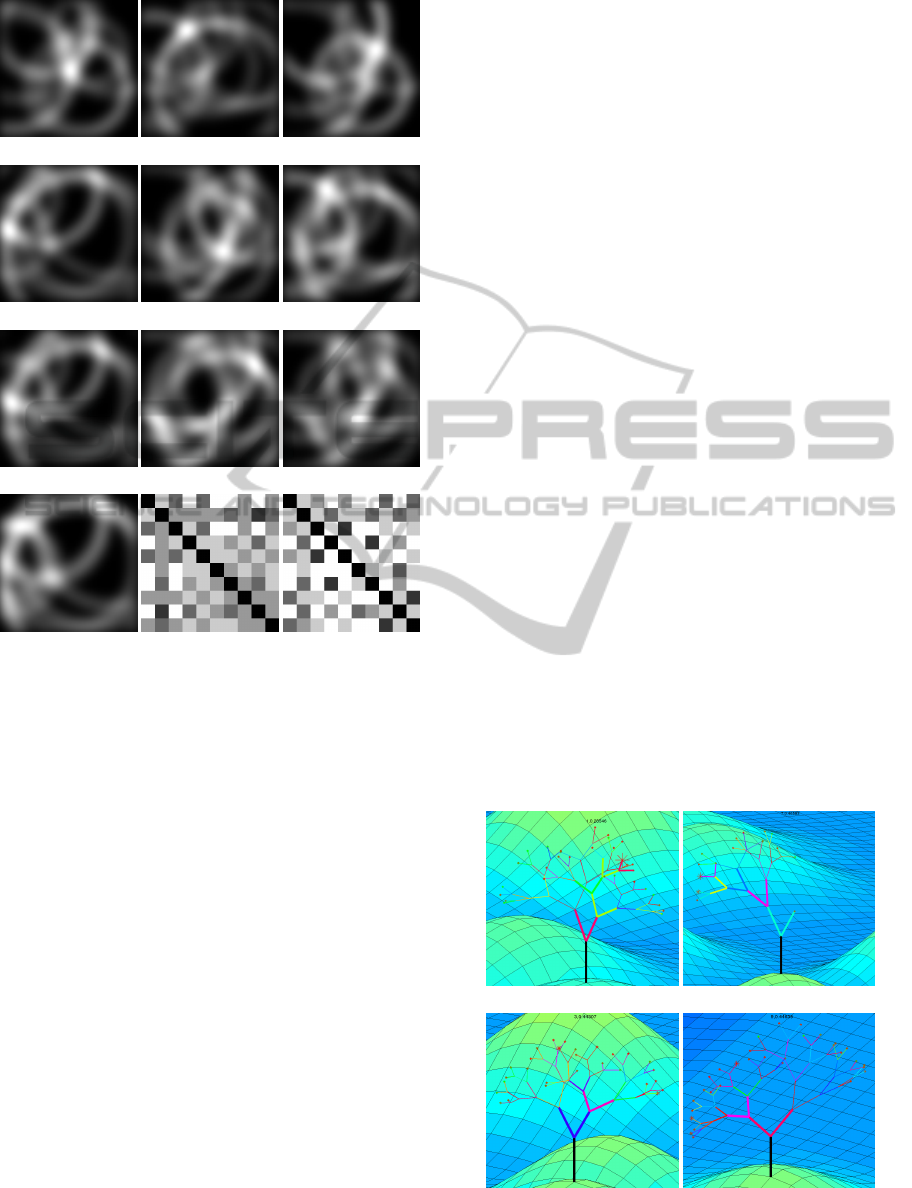
4.1 Single Trees
Figure 3 shows four different examples of a Random
Forest, where the maximal tree height was set to five,
only one test per node is created, and the split point
(i.e. θ in Equation 1) is sampled uniformly from the
interval defined by the minimal and maximal values
of the randomly selected data dimension. The trees
show extremely weak performance with an average
0-1-loss of 57%. Figure 3 gives a visual explanation
for one of the major reasons for this low accuracy:
The approach of creating only one test and to uni-
formly sample the split point does not perform any
task-specific optimization. Consequently, there is a
(a) (b)
(c) (d)
Figure 3: Extremely weak trees (Maximal height: 5; Uni-
form sampled split point; One test per node).
PerformanceAssessmentandInterpretationofRandomForestsbyThree-dimensionalVisualizations
153
very high risk of creating a weak split, i.e. a split
which propagated only a small fraction of the data to
one of the child nodes. Since the maximal tree height
is set to five, only a few splits are possible. If most of
them are unbalanced, very large and impure leaves are
created which contain the major part of the data. Fig-
ure 3(a)-3(b) show examples of this problem. Even if
the created splits are more or less balanced, there are
too few of them (due to the small maximal tree height)
and they are too less optimized (due to uniform sam-
pled split points). Figure 3(c)-3(d) show examples of
such trees, where the leaves are of similar size but
with high impurity.
(a)
(b)
Figure 4: Strong trees (Maximal height: 45; Uniform sam-
pled split point; One test per node).
One possible solution for this problem is to simply
increase the maximal tree height. Figure 4 shows
two exemplary trees of a Random Forest, where the
maximal tree height was increased to 45, while the
remaining parameters stayed unchanged. There are
still imbalanced splits as for example the split of the
root node in Figure 4(b). However, due to the consid-
erably higher maximal height, there are enough pos-
sibilities to create well-balanced splits. The number
of impure leaves does consequently decrease dramat-
ically, while the strength increases (the 0-1-loss falls
from 57% to 39%). Nevertheless, there are still a con-
siderable amount of unbalanced splits (see e.g. first
branches of tree in Figure 4(b)) as well as weakly op-
timized leaves (many small, red leaves in Figure 4(a)).
(a)
(b)
Figure 5: Strong trees (Maximal height: 45; Gini-optimized
split point; One test per node)
The small size of the leaves of the trees depicted in
Figure 4 indicate, that the performance of the RF
cannot be further increased by increasing the max-
imal height of its trees. Instead, a larger amount
of optimization has to be introduced during tree in-
duction. One way to achieve that is to optimize the
split point with respect to the impurity of the result-
ing child nodes instead of selecting it randomly. The
Gini-impurity (Equation 3) is commonly used for this
purpose. This decreases the risk of selecting weak
split points and can lead to an increase of perfor-
mance. The trees in Figure 5 have been created with
the Gini-optimized split point selection and a maxi-
mal tree height of 45. They show considerably less
red leaves than the trees in Figure 4. However, it does
not change the risk of selecting a bad splitting dimen-
sion as is illustrated in Figure 5(b) (first splits after
root node).
IVAPP2015-InternationalConferenceonInformationVisualizationTheoryandApplications
154

(a) (b)
(c)
Figure 6: Very strong trees (Maximal height: 45; Median-
based split point; Ten tests per node).
Figure 6 shows three examples with the highest de-
gree of optimization used in this section. The split
point is defined as the median of the data in each node,
which leads to very balanced splits. The maximal tree
height was set to 45 allowing for as many (balanced)
splits as possible for the used dataset and a maximal
information extraction. Furthermore, each node cre-
ated ten different tests (i.e. selected ten different split-
ting dimensions) and selected the best split (based on
the Gini-impurity of the child nodes). Consequently,
the individual nodes as well as the whole tree is rela-
tively balanced, as can be seen in Figure 6. The indi-
vidual strength (measured as 1 − E
01
) of these trees is
with 0.8 the highest of all tree examples of this sec-
tion, which is illustrated by the high hills on which
the trees are located.
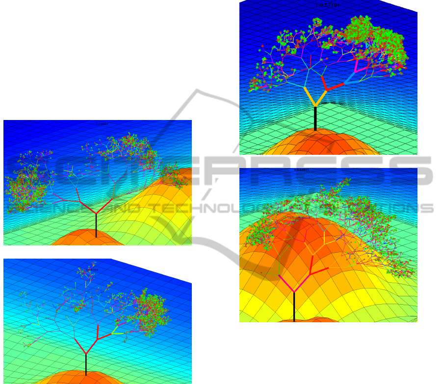
4.2 Forest
While the previous section discussed properties of in-
dividual trees, the current section brings these trees
into the context of the whole forest. Each tree is al-
ready given with its 3D layout, which is controlled
by the recursive splitting process during tree induc-
tion (shape/color of the tree), the impurity of the leaf
nodes after tree training (color/size of leaves), as well
as the strength of the tree measured as out-of-bag 0-1-
loss during tree evaluation (height of the local hill of
the tree). The two properties that remain to be visual-
ized are the strength of the whole forest as well as the
correlation between the individual trees.
(a) Maximal height: 5; Uniform sampled split
point; One test per node
(b) Maximal height: 15; Uniform sampled
split point; One test per node
(c) Maximal height: 45; Uniform sampled
split point; One test per node
(d) Maximal height: 15; Gini-optimized split
point; One test per node
(e) Maximal height: 5; Median-based split
point; Ten tests per node
(f) Maximal height: 45; Median-based split
point; Ten tests per node
Figure 7: Forest examples.
PerformanceAssessmentandInterpretationofRandomForestsbyThree-dimensionalVisualizations
155

Figure 7(a)-7(c) show RFs with uniform sampled split
points, one test per node, and a maximal tree height
of 5, 15, and 45, respectively. Four key characteristics
of the increase of the maximal tree height are imme-
diately evident: 1) The decision trees become larger
and more complex as visualized by height and shape
of the displayed trees. 2) The trees become stronger
as visualized by the height of the local hill (0-1-loss
decreases from 54% to 39%). 3) The performance of
the whole RF increases as well (BA increases from
54% to 93%), which is visualized by the height of
the global plateau. 4) The trees correlate more and
more with each other (average correlation increases
from 0.4 to 0.84) and are consequently located closer
to each other.
Figure 7(d) shows an RF with Gini-optimized split
point selection and a maximal tree height of 15. Com-
pared to an RF with similar parameter setting but uni-
form sampled split points, the performance increased
from 66% to 71%, which is visualized by a slightly
higher plateau. Figure 7(e)-7(f) show an RF with
median-based split point definition, best-of-ten test
selection, as well as a maximal tree height of 5 and
45, respectively. The advantage of this tree induc-
tion scheme is immediately evident if the visualiza-
tion in Figure 7(e) is compared to the visualizations
of the other RFs of this section. Already at this shal-
low maximal tree height, it outperforms other RFs as
can be clearly seen by the height of the global plateau
and local hills. Both, individual as well as global
performance, increase with higher trees: The BA in-
creases from 90% to 95% (leading to a slightly higher
plateau in Figure 7(f) than in Figure 7(e)). The aver-
age strength of the trees increases, i.e. the tree error
decreases from 0.28 to 0.20 (resulting in higher lo-
cal hills). Also the correlation increases from 0.79 to
0.92 on average, which leads to a very dense forest in
Figure 7(f). Figure 8(a)-8(b) visualize the same RF as
in Figure 7(f) from different viewing directions.
(a) (b)
Figure 8: Different views of one forest (Maximal height:
45; Median-based split point; Ten tests per node).
5 CONCLUSIONS
This work introduced a novel technique to visual-
ize one of the most successful machine learning ap-
proaches. Unlike other methods to visualize certain
properties of Random Forests, the current work is nei-
ther completely abstract, nor completely data-driven,
but instead combines both categories to a exemplar-
driven visualization. Besides only illustrating the un-
derlying principle of decision trees, it visualizes a spe-
cific, given Random Forest. Many of the main prop-
erties of a Random Forest including individual tree
strength and correlation as well as the strength of the
whole forest are dominant visual characteristics and
allow a fast and accurate judgement of the general
performance of the underlying RF classifier. An anal-
ysis of shape and color of the individual trees allows
to infer knowledge about unfavorable parameter set-
tings and provide cues for adjustments in order to in-
crease performance.
Future work will mainly focus on a higher ad-
vanced graphical user interface, which allows to blend
in more information about the Random Forest at hand
and to switch easily between different modes of visu-
alization (e.g. single tree, 1D sorted trees, spatially
arranged trees, etc.). Furthermore, an online visual-
ization which visualizes the RF during tree induction
and training can be beneficial to gain an even deeper
understanding of the learning part which eventually
might lead to new theoretical insights about RFs in
particular and EL in general.
REFERENCES
Breiman, L. (1996). Bagging predictors. In Machine Learn-
ing, pages 123–140.
Breiman, L. (2001). Random forests. Machine Learning,
45(1):5–32.
Geurts, P. and Wehenkel, D. E. L. (2006). Extremely ran-
domized trees. Machine Learning, 63(1):3–42.
H
¨
ansch, R. (2014). Generic object categorization in PolSAR
images - and beyond. PhD thesis.
Rodriguez, J. J., Kuncheva, L. I., and Alonso, C. J. (2006).
Rotation forest: A new classifier ensemble method.
IEEE Transactions on Pattern Analysis and Machine
Intelligence, 28(10):1619–1630.
Shotton, J., Johnson, M., and Cipolla, R. (2008). Semantic
texton forests for image categorization and segmen-
tation. In IEEE Conference on Computer Vision and
Pattern Recognition, pages 1–8.
Zeiler, M. D. and Fergus, R. (2014). Visualizing and under-
standing convolutional networks. In Computer Vision
ECCV 2014, volume 8689 of Lecture Notes in Com-
puter Science, pages 818–833.
IVAPP2015-InternationalConferenceonInformationVisualizationTheoryandApplications
156
