
Route Segmentation into Speed Limit Categories by using Image
Analysis
Philippe Foucher, Emmanuel Moebel and Pierre Charbonnier
Cerema/DTer Est/LR Strasbourg, ERA 27, 11 rue Jean Mentelin, BP9, 67035 Strasbourg, France
Keywords:
Road Scene Classification, Speed Limits, Image Analysis, Route Segmentation, Evaluation.
Abstract:
In this contribution, we address the problem of road sequence segmentation into speed limit categories, as
perceived by the user. We propose an algorithm that is based on two processing steps. First, the images are
classified independently using a standard random forest algorithm. Low-level and high-level approaches are
proposed and compared. In the second phase, a sequential smoothing of the results using different filters is
applied. An evaluation based on two databases of images with ground truth shows the pros and cons of the
methods.
1 INTRODUCTION
Historically, most vision-based road scene analysis
systems have been dedicated to detecting and recog-
nizing components of the scene, such as pedestrians,
cars, obstacles, signs, or road markings. In this pa-
per, we address a more recent application of image
analysis, which aims at classifying the road scene, as
a whole, into a semantic category. Applications are
related to the research about self-explaining roads, in
which driving psychologists investigate about the re-
lationships between visual characteristics of the road
and its environment and road “readability” (Charman
et al., 2010). In other words, the mental categorization
of roads is known to have an impact on the driver’s
behavior. Hence, road legibility should be diagnosed
and enhanced by appropriate treatments of the infras-
tructure, to improve road safety. For the moment,
these works are based on the analysis of road im-
age sequences by human operators, which represents
a considerable work at the scale of a road network (in
our application, image sequences are collected by an
inspection vehicle along itineraries, typically one im-
age every 5 meters).
In this work, we investigate the segmentation of
routes into speed limit categories, as perceived by the
user. Among the six speed limits defined in the French
regulations, we here consider 4 categories : 50 km/h ;
70 km/h ; 90 km/h and 110 km/h. Note that, in France,
speeds are limited to 50 km/h in built-up areas, 110
km/h on dual carriageway roads, that are separated
by a central island or barrier and 90 km/h on rural
two-way roads. In some dangerous situations, such as
crossings, driving speeds are limited to 70 km/h (so
this class is difficult to discriminate based on visual
cues only, even for human operators). Sample images
of the 4 categories are shown on fig. 1.
As a first contribution, we propose a two-step cat-
egorization method. The first step relies on a classi-
fication of individual images, which is performed us-
ing either a low-level approach or a high-level scheme
based on an intermediate representation of the scene.
Note that, in both cases, the classification into four
categories is obtained using the random forest algo-
rithm (Breiman, 2001). Of course, analyzing images
individually is inappropriate, so the second step of the
proposed method consists in a sequential smoothing
of the classification results to obtain a consistent route
segmentation. The second contribution of the paper is
that we perform a systematic evaluation of the algo-
rithm on large image databases.
The rest of the paper is organized as follows. We
first propose a short review of related works in Sect. 2.
Then, in Sect. 3, we describe the algorithm for clas-
sifying images into speed limit categories. In Sect. 4,
the experimental setup is presented. In Sect. 5, we
comment the experimental results. Sect. 6 is dedi-
cated to conclusions and future works.
2 RELATED WORK
Different approaches have been proposed to classify
natural scenes into semantic categories. We refer the
416
Foucher P., Moebel E. and Charbonnier P..
Route Segmentation into Speed Limit Categories by using Image Analysis.
DOI: 10.5220/0005312704160423
In Proceedings of the 10th International Conference on Computer Vision Theory and Applications (VISAPP-2015), pages 416-423
ISBN: 978-989-758-090-1
Copyright
c
2015 SCITEPRESS (Science and Technology Publications, Lda.)
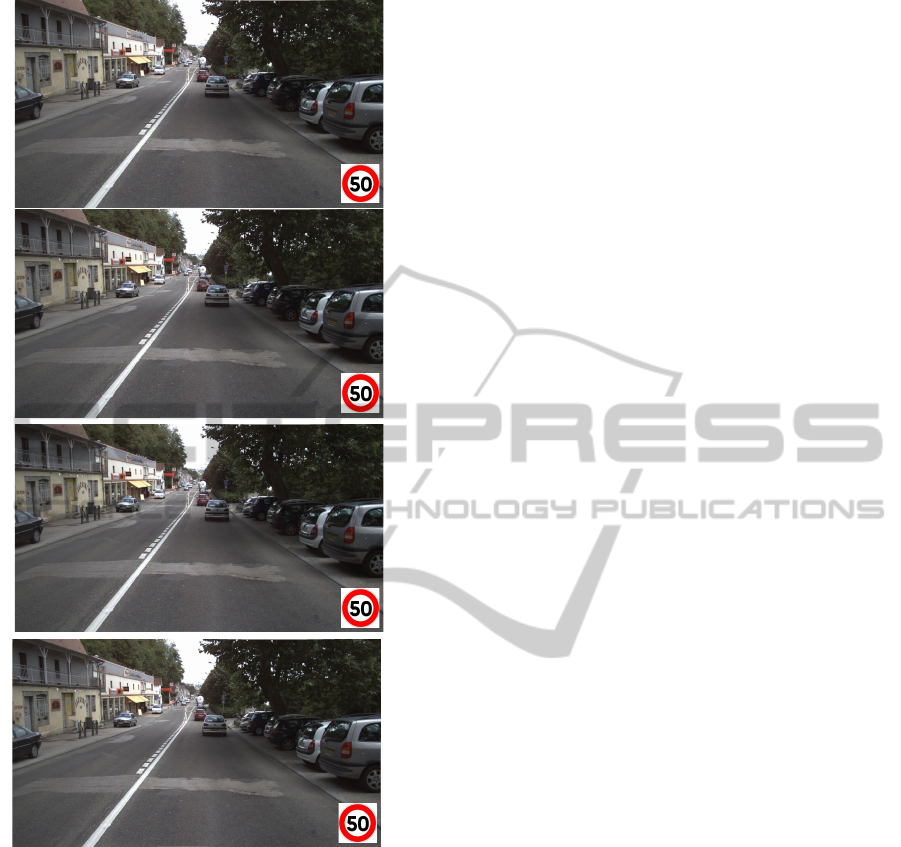
Figure 1: Examples of speed limit categories.
reader to (Bosch et al., 2007) for a global review of
scene classification strategies. In a first approach,
the classification is based on statistical learning us-
ing low-level visual features, such as color, edges or
textures, i.e. images are classified without any seman-
tic knowledge of the objects in the scene. In (Vailaya
et al., 1998), the classification of outdoor images into
“city” or “landscape” category is based on color and
edge directions features. Experiments show that edge
direction features are discriminative enough to be
used alone in the algorithm. In (Wu and Rehg, 2011),
the CENTRIST(CENsus TRansform hISTogram) de-
scriptor was introduced and assessed on five graylevel
image data sets, including scene recognition data. The
use of CENTRIST improves the classification per-
formances compared to other usual descriptors. It
may be noticed that the mCentrist descriptor, a multi-
channel version of CENTRIST, has been recently in-
troduced (Xiao et al., 2014). On four image data sets
(indoor and outdoor images), the authors have shown
that mCentrist enhances the performances of CEN-
TRIST in terms of scene classification.
In a second approach, an intermediate repre-
sentation of the scene is built in order to bridge
the semantic gap between low-level descriptors and
high-level semantic information. The bag-of-words
(BOW) approach is commonly used to obtain a se-
mantic model of the image. In this framework, im-
ages are represented by histograms of visual words,
which are generated from local image patches by
some unsupervised classification algorithm using
SIFT (Lowe, 1999) or histograms of oriented gradi-
ent (HOG) (Dalal and Triggs, 2005) as input features.
These histograms of visual words are then consid-
ered as high-level attributes for scene classification.
In (Bosch et al., 2007), a methodology has been pro-
posed to compare the performances of the low-level
and high-level strategies. The authors have shown that
the use of an intermediate semantic modeling is more
appropriate when the number of categories is high and
in the presence of ambiguities between classes. In
contrast, low-level features can be useful when the
number of semantic categories is low and when the
categories are easily distinguishable. The computa-
tion time is also lower.
We may note that, among the numerous existing
scene classification works, only a few are dedicated
to the particular case of road scenes. A scheme, based
on low-level color and texture features, is proposed
to classify road driving environment into four differ-
ent categories (off-road, major road, motorway, ur-
ban road) in (Tang and Breckon, 2010; Mioulet et al.,
2013). The aim of this research is to propose an au-
tonomous sensor to adapt the vehicle dynamics (trac-
tion, braking, engine dynamics) to the driving envi-
ronment and the descriptors are computed in three
regions of interest, selected to extract relevant prop-
erties of the road and its surroundings. Road scene
understanding is also investigated in (Ess et al., 2009)
to identify road type. This research is focused on ur-
ban road scenes and the authors propose a two-step
method. A supervised learning process is first used
to segment images into semantic objects (walls, road,
cars, grass...) and a classification algorithm is then
applied to identify 8 road types and detect the pres-
ence of 3 kinds of objects (cars, pedestrians, pedes-
trian crossing).
In the literature, to our knowledge, there is no
paper that concerns the classification of images into
RouteSegmentationintoSpeedLimitCategoriesbyusingImageAnalysis
417
speed limit categories. The closest work to our con-
tribution is probably Ivan and Koren’s paper (Ivan
and Koren, 2014) in which the authors propose to
automatically classify road scenes as built-up and
non-built-up areas using a bag-of-words methodol-
ogy. However, our approach differs in the number of
categories and, moreover, we smooth the scene clas-
sification results along the sequence to obtain a rel-
evant route segmentation. Note that, in (Ess et al.,
2009), the effect of temporal smoothing using Markov
Random Fields (MRF) in the segmentation process is
evaluated, showing the benefits of using sequential in-
formation. However MRF’s are not used in the scene
classification step due to computational limitations.
3 PROPOSED METHOD
Our method aims at classifying images into four
speed limit categories. It is a two-step algorithm with
an image classification phase and a post-processing
phase that smoothes the results by considering the ar-
rangement of the images in a temporal sequence.
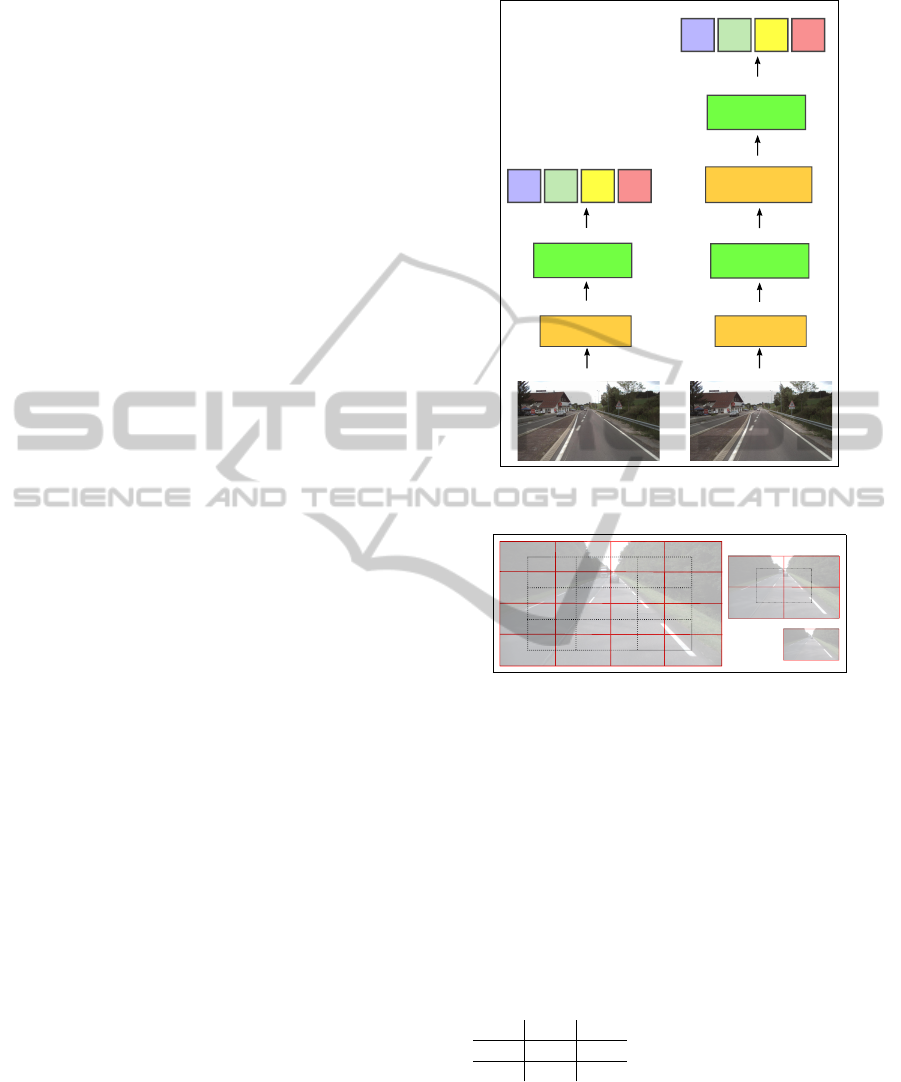
3.1 Image Classification Algorithms
We propose in fact two algorithms, based either
on low-level features or on a high-level representa-
tion, as summarized in Fig. 2. In both cases, the
scene is classified using the random forest meta-
classifier (Breiman, 2001).
A random forest is an ensemble of decision trees
that predict a class from a set of features. The predic-
tion of a tree is obtained by using successive binary
decision rules. Every tree is learned independently on
a randomly selected sample of features of the training
data set, with replacement (bootstrap process). The
result of the random forest algorithm is a probabil-
ity which is obtained by combining the outputs of the
trees. A sample is assigned to the class that corre-
sponds to the maximum probability. Note that ran-
dom forests are intrinsically multi-class and can be
easily parallelized. The input features of the random
forest differ between our low-level and high-level ap-
proaches. In the low-level algorithm, mCentrist fea-
tures are computed directly from the image. In the
second approach, the features are extracted from an
intermediate representation of the image, previously
generated using a clustering algorithm.
3.1.1 Low-level Approach: Centrist and
mCentrist Features
The Centrist descriptor (Wu and Rehg, 2011) is an
mCENTRIST
Low-level features
HOG
Low-level features
Image Image
Random forest
Scene classification algorithm
110
90
70
50
Speed limit categories
Random forest
Scene classification algorithm
110
90
70
50
Speed limit categories
high-level features
Histograms
of visual words
k-means
Intermediate representation
Figure 2: Scene classification methodology: low-level (left)
and high-level (right) approaches.
Figure 3: Spatial pyramid with levels 2, 1 and 0. For ex-
ample, the level 2 representation (left image) is split into 25
blocks : 16 red blocks (continuous lines) and 9 black blocks
(dash lines). There is an overlap of 25% between red blocks
and blacks blocks.
histogram of the Census Transform (CT) val-
ues (Zabih and Woodfill, 1994). The CT value, which
is akin to a Local Binary Pattern (LBP (Ojala et al.,
1996)), corresponds to a byte that encodes the com-
parisons between the current pixel and its eight neigh-
bours. More specifically, a bit is set to 1 if the pixel is
higher than (or equal to) the central pixel, else it is set
to 0. Neighbours are searched from left to right and
from top to bottom:
156 168 172
156 156 157
153 150 155
⇒ (10010111)
2
⇒ CT = 151 (1)
Spatial information is incorporated into the fea-
tures by using a pyramid. In this scheme, multi-scale
representations of the image are obtained by divid-
ing it into several blocks, from which the Centrist
descriptors are extracted. We use a 2-level pyramid
with 31 blocks, as proposed in (Wu and Rehg, 2011).
Note that the blocks are built with identical dimen-
VISAPP2015-InternationalConferenceonComputerVisionTheoryandApplications
418

156156 157
168156 172
150153 155
Channel 1
135135 137
134136 122
141135 145
Channel 2
156
156 172
153 155
156156 157
168
150
135
136
122
135 145
135135 137
134
141
mCT
1
=(10110110)
2
=(182)
10
{
{
mCT
2
=(01011100)
2
=(92)
10
{
{
Figure 4: mCentrist computation by combining 2 channels.
sions and with an overlap of 25% between successive
scales (see Fig 3).
Color information, that is ignored in the Centrist
descriptor, can be dealt with using mCentrist, a multi-
channel extension of Centrist, proposed in (Xiao
et al., 2014), in which channels are combined pair-
wise as shown on Fig. 4. In our contribution, we
consider a 4-channel color space (three channels in
opponent color space and a Sobel contour image), as
in (Xiao et al., 2014).
In Sect.5, we experimentally evaluate the influ-
ence of color and spatial information.
3.1.2 High-level Approach
In our bag-of-words approach, HOG (Dalal and
Triggs, 2005) are first extracted from rectangular re-
gions of interest (ROI) placed on a regular grid on the
image. The number of bins n
bins
of the HOG is usu-
ally a sub-multiple of 180
◦
. The optimal value we
found in our experiments is given in Sect. 5. It may
be noticed that, since we use HOG features, color in-
formation is ignored at this step. The k-means algo-
rithm is then used to generate a codebook by cluster-
ing the features into visual words. The random for-
est algorithm, with the histogram of words as input
features, is finally applied to classify the scene into a
speed limit category. The size of the patch, n
c
× n
c
pixels, and the number of words n
words
in the visual
vocabulary are empirically determined and the results
are shown in Sect 5.
3.2 Route Segmentation
We are interested in segmenting routes into homoge-
neous road sections according to a speed limit crite-
rion. The classification should be more robust and
relevant by taking into account the image sequence
than by using images individually. Considering the
posterior probabilities over the sequence as a 1-D sig-
nal, we propose to smooth the outputs of the classifier
by applying successively a mean filter and a morpho-
logical filter (Serra and Vincent, 1992) over the sig-
nal. The two filters aim at eliminating the small seg-
ments in the sequence. The number N
f ilter
of neigh-
boring images centered on the current image varies
over the range [0,100]. We remind the reader that 100
images correspond to 500 meters. The mean filter is
first applied to the probabilities stemming from image
classification. The four mean signals are then filtered
by morphological closing and morphological opening
operations and normalized. The structuring element
of the morphological filter is a vector of dimension
N
f ilter
× 1. Finally, the image is assigned to the class
of maximum filtered probability.
4 EXPERIMENTAL SETUP
We consider real-world image sequences acquired by
frontal cameras mounted on top of inspection vehi-
cles. Images are taken every 5 meters during day-
time under various, uncontrolled lighting conditions.
The image size is 1920 × 1080. We will consider two
kinds of data sets : individual images data set and se-
quence data set. Every image of the data sets is man-
ually given a speed limit label in order to establish a
ground truth (GT).
4.1 Individual Images Data Set
This data set is composed of 640 individual images
(i.e. no sequential information is considered) equally
split into the four categories. This data set is used
for the training phase, for the determination of low-
level features and for the empirical optimization of
the BOW parameters n
bins
, n
c
and n
words
in the high-
level approach.
4.2 Sequence Data Set
The sequence data set comprises 11689 images with
homogeneous sections of the different speed limit cat-
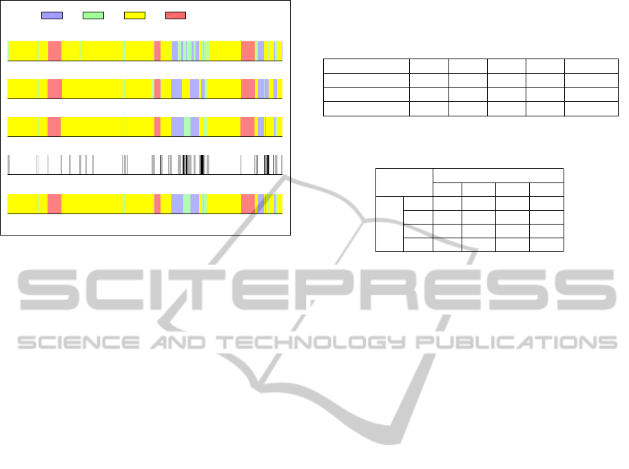
egories. Three different human operators have built
three GT’s (GT1, GT2 and GT3) according to their
visual perception of the scenes, as illustrated in Fig. 5.
Note that the number of images by category is highly
imbalanced, with a majority (68%) of images in the
90 category. We quantify that 14.04% (respectively
11.16% and 9.06%) of the images have been catego-
rized differently in GT1 and GT2 (respectively GT1-
GT3 and GT2-GT3). The differences between ground
truths are mainly located at the transitions between
categories. However, we observe other ambiguities,
often corresponding to sections that are categorized
RouteSegmentationintoSpeedLimitCategoriesbyusingImageAnalysis
419
1000 2000 3000 4000 5000 6000 7000 8000 9000 10000 11000
Ground truth 1
Image number
1000 2000 3000 4000 5000 6000 7000 8000 9000 10000 11000
Ground truth 2
Image number
1000 2000 3000 4000 5000 6000 7000 8000 9000 10000 11000
Ground truth 3
Image number
1000 2000 3000 4000 5000 6000 7000 8000 9000 10000 11000
Ground truth differences
Image number
1000 2000 3000 4000 5000 6000 7000 8000 9000 10000 11000
Final ground truth for evaluation
Image number
50 70 90 110
Figure 5: Ground truths for the sequence data set. The ab-
scissa represents the image number. Colors correspond to
labels (50 ; 70 ; 90 ; 110). The rows 1-3 are the 3 GT.
The fourth row shows the ambiguities between GT’s: white
means no difference between GTs ; gray means that a GT
differs from the two others; black means that the 3 GT’s are
different. The last row corresponds to GT
eval
.
as 70 by one (or two) operator(s). To evaluate the per-
formances of the algorithms, we build a single ground
truth (GT
eval
) by combining GT1, GT2 and GT3. The
majority category in GT1, GT2 an GT3 is allocated
to GT
eval
. When we observe three different labels
(1.82% of the images), the median label is assigned
to GT
eval
.
5 RESULTS AND DISCUSSION
In this section, the individual images data set is used
to compare the performances with Centrist and mCen-
trist descriptors (§ 5.1) and to determine the best val-
ues n
bins
, n
c
and n
words
for the BOW approach (§ 5.2).
Note that the classification rate is calculated by cross-
validation. The image classification algorithms are
then tested on the sequence data set and the impact of
sequential smoothing is analyzed (§ 5.4). Throughout
the current section, the number of trees in the random
forest is 200 for the low-level approach and 300 for
the high-level approach.
5.1 Considering Centrist, mCentrist
and Spatial Pyramid
In this experiment, we evaluate the classification on
the individual images data set by using Centrist and
mCentrist with or without spatial information in the
low-level approach. The results are gathered in tab. 1.
Table 1: Scene classification into four speed limit categories
by low-level approach. Results (true positive rate in %) on
image data set by using Centrist, mCentrist and mCentrist +
Spatial Pyramid (SP).
features 50 70 90 110 Overall
Centrist. 90.0 78.1 67.5 84.4 79.6
mCentrist 90.6 78.8 74.4 86.9 82.7
mCentrist+SP 95.0 79.4 83.8 96.2 88.7
Table 2: Confusion matrix (in %) for the low-level ap-
proach.
Algorithm results
50 70 90 110
GT
50 95 5 0 0
70 10 79.4 10 0
90 1.9 9.4 83.8 5
110 0 1.9 1.9 96.2
We distinguish the true positive rate (TPR) by cat-
egory from the overall score, which is the mean of
TPR for the four categories. By analyzing the results,
it may be noticed that the use of color information
has a strong impact for the classification into the cate-
gory 90 (the TPR increases by 10.2% with mCentrist).
The improvements of performances with mCentrist
are less significant for the other categories. The TPR
increases respectively by 0.7%, 0.9% and 2.9% for the
categories 50, 70 and 110. It may be explained by the
nature of the images in the category 90 which mainly
contains rural images with typical color objects (veg-
etation, forests). The use of the spatial information
has a great influence on the classification scores for
all categories, except category 70 (for which the im-
provement is low). The TPR using mCentrist and SP
are much higher than the TPR using mCentrist on the
whole image. Hence, we retain the mCentrist descrip-
tors computed on the blocks of spatial pyramid in the
rest of our experiments. The confusion matrix of the
low-level approach using mCentrist and SP is given
in Tab 2. Note that the TPR of the categories 50 and
110 are much higher than the TPR of the intermediate
categories 70 and 90. For these two intermediate cat-
egories, the misclassifications are due to confusions
between the category 70 and 90. About 10% (resp.
9.4%) of images in the category 70 (resp. 90) in GT
are classified in the category 90 (resp. 70).
5.2 Bag-of-Words Optimization
We focus on the determination of the values n
bins
,
n
c
and n
words
with a series of experiments using the
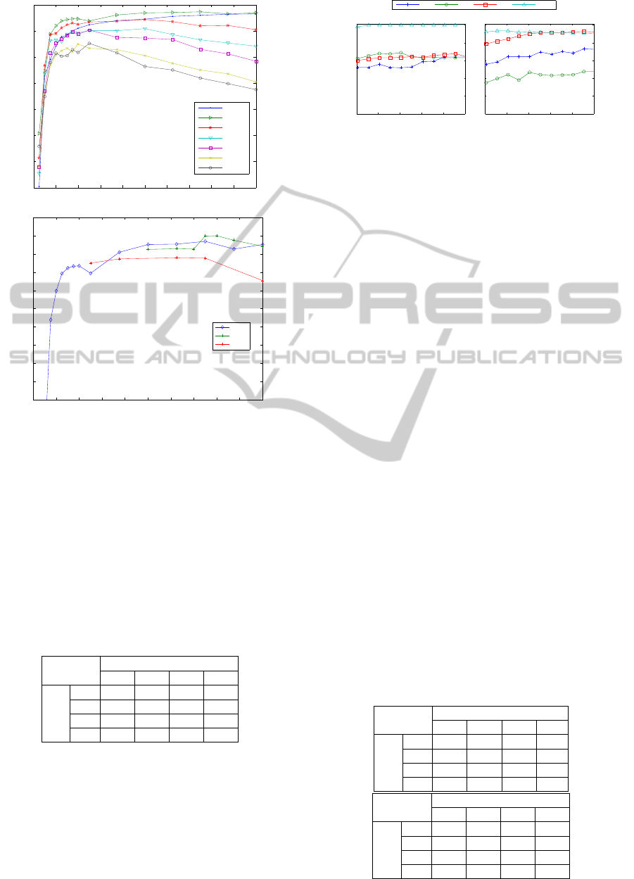
individual images data set. The curves plotted on
Fig. 6 show the overall TPR vs. the number of words
(n
words
) either for several values of n
c
(top) or for
three values of n
bins
(bottom). In Fig. 6-top, we ob-
VISAPP2015-InternationalConferenceonComputerVisionTheoryandApplications
420
0 20 40 60 80 100 120 140 160 180 200
50
55
60
65
70
75
80
85
Overall true positive rate (%)
number of words (n
words
)
n
c
=10
n
c
=20
n
c
=30
n
c
=40
n
c
=50
n
c
=60
n
c
=70
0 20 40 60 80 100 120 140 160 180 200
75
76
77
78
79
80
81
82
83
84
85
number of words (n
words
)
Overall true positive rate (%)
n
bins
=9
n
bins
=18
n
bins
=36
Figure 6: Overall TPR vs. the number of words in codebook
(in abscissa) for several sizes of patches n
c
(top) and for
three for three values of n
bins
in HOG (bottom).
serve that the TPR with n
c
= 20 (and n
bins
= 9) is sys-
tematically higher than the six other values whatever
the number of words. We chose this value for the sec-
ond experiment (Fig. 6-bottom) in which the number
of bins is evaluated. We can see that the best perfor-
mances are obtained with n
bins
= 18 for n
words
= 160.
Hence, these values are chosen for the remaining of
the paper.
Table 3: Confusion matrix (in %) for the BOW approach.
Algorithm results
50 70 90 110
GT
50 90.6 8.1 0.6 0.6
70 7.5 81.2 10 1.2
90 1.2 5.6 88.8 4.4
110 0.6 0.6 1.9 96.9
5.3 Comparison Between Low-level and
High-level Approaches
The confusion matrix of BOW algorithm, applied to
the individual images data set, is shown in Tab. 3.
It may be noticed that, for the category 90 and 70,
the high-level method (TPR = 88.8% and 81.2%)
0 20 40 60 80 100
0
20
40
60
80
100
Low−level approach
N
filter
True positive rate (%)
0 20 40 60 80 100
0
20
40
60
80
100
High−level approach
N
filter
True positive rate (%)
50 70 90 110
Figure 7: TPR vs. the number of images for the
filters:N
f ilter
.
performs better than the low-level algorithm (TPR =
83.8% and 79.4%). On the other hand, the category
50 is better identified using mCentrist features than
using bag-of-words model. In both cases, the lower
performances are obtained for the category 70. In
terms of computation time, the mCentrist extraction
takes 4.2 seconds per image while the bag-of-words
extraction is longer (10.1 seconds per image).
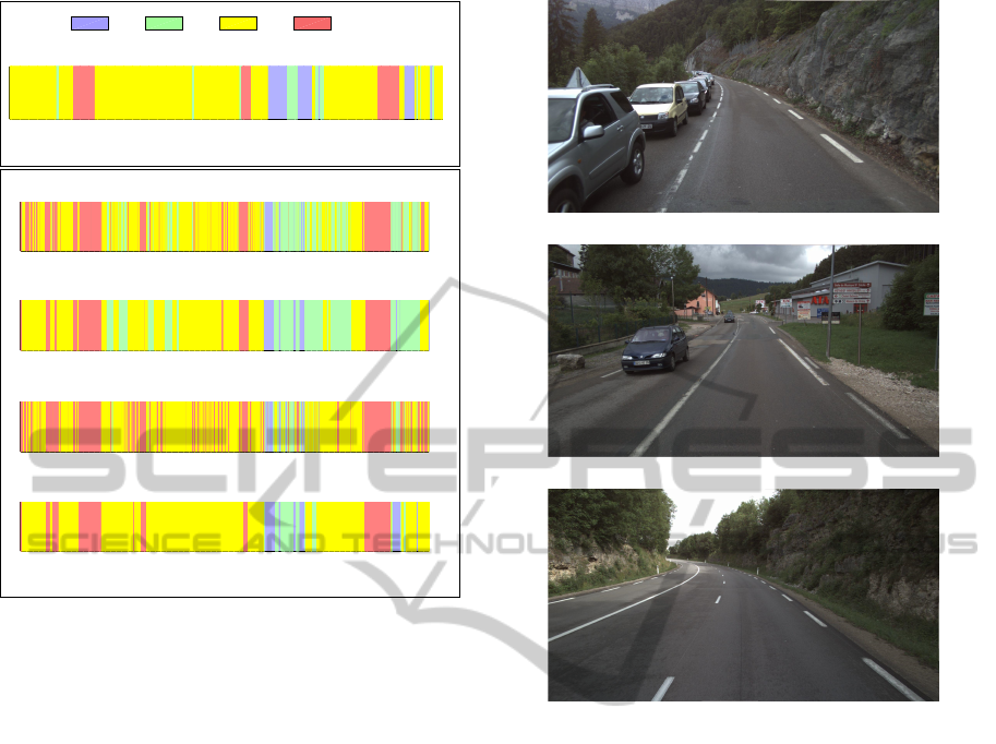
5.4 Evaluation of Route Segmentation
Algorithm
In this section, we evaluate the route segmentation
method on the sequence data set. A smoothing, as
described in Sect. 3, is applied on the results of the
image classification. The results of route segmenta-
tion without filtering are shown on Fig. 8. By visually
comparing the classification using either low-level ap-
proach (Fig 8-2
nd
row) or high-level approach (Fig 8-
4
th
row) to the ground truth (Fig 8-1
st
row), we note
that the road sections are coarsely identified. How-
ever, we observe a lot of category changes between
successive images. This confirms that it it necessary
to smooth the individual classification results using
neighboring results. The size of the filter N
f ilter
, cen-
tered on the current image, can be empirically de-
termined. The curves TPR by category vs. N
f ilter
Table 4: Confusion matrix (in %) for the route segmenta-
tion algorithm : (top) mCentrist approach ; (bottom) BOW
approach. N
f ilter
= 21.
Algorithm results
50 70 90 110
GT
50 55.7 44.3 0 0
70 5.1 67.6 27.1 0.1
90 0.4 27.6 62.9 9
110 0 0 0 100
Algorithm results
50 70 90 110
GT
50 64.4 25.3 6.3 4
70 4.3 44.1 51 0.1
90 0.3 4 84.5 11.1
110 0 0 6.5 93.5
RouteSegmentationintoSpeedLimitCategoriesbyusingImageAnalysis
421
1000 2000 3000 4000 5000 6000 7000 8000 9000 1000011000
GT
eval
Image number
50
70 90 110
1000 2000 3000 4000 5000 6000 7000 8000 9000 1000011000
mCentrist
Image number
1000 2000 3000 4000 5000 6000 7000 8000 9000 1000011000
mCentrist + smoothing
Image number
1000 2000 3000 4000 5000 6000 7000 8000 9000 1000011000
BOW
Image number
1000 2000 3000 4000 5000 6000 7000 8000 9000 1000011000
BOW + smoothing
Image number
Figure 8: Route segmentation algorithm for the sequence
data set. The abscissa represents the image number in the
sequence. Colors correspond to the label (50 ; 70 ; 90 ;
110). The first row is the ground truth GT
eval
as defined
in Sect. 4. The next two rows are the segmentation using
the low-level approach without (row 2) and with (row 3)
smoothing. The last two rows are the segmentation using
the high-level method without (row 4) and with smoothing
(row 5). N
f ilter
= 21.
are plotted on Fig 7. N
f ilter
varies over the range
[0,100]. The value 0 means that smoothing is dis-
abled. A study of these curves shows that the im-
provement of performances with smoothing is signif-
icant for the two approaches whatever N
f ilter
. The in-
crease for the high-level approach is higher than for
the mCentrist method. No value N
f ilter
gives the op-
timum for all categories. We propose to use a rather
low value N
f ilter
= 21 to reduce the smoothing impact
in the algorithm. Quantitative performances are gath-
ered in Table 4. It may be noticed that the results for
the sequence data set are lower than the TPR for the
individual images data set (see tab. 2, 3). Both algo-
rithms perform very well to classify images into the
category 110. In the mCentrist approach, The TPR
are quite homogenous for categories 50 (TPR=55.7%)
, 70 (TPR=69.6%) and 90 (TPR=62.7%). We observe
a lot of confusions between the three categories. The
performances using BOW are quite better in the cate-
gory 50 and much higher in the category 90 by com-
paring to the mCentrist approach. On the other hand,
(a)
(b)
(c)
Figure 9: Examples of false classifications : (a) image clas-
sified as 50 by the low-level method and as 90 by BOW, as
in GT
eval
; (b) ambiguous situation. The image is identified
as 90 in GT; (c) image wrongly classified as 110.
the TPR is very low in the category 70 (TPR=44.1%).
It may be noticed that the categories 50, 70 and 90
represent variable situations (as shown in Fig 9-a and
b, both images illustrate scene in category 90). The
category 110 is more homogenous. This could ex-
plain that the performances are different for the cat-
egory 110 with respect to the three others. Figure 8-
(3
rd
and 5
th
row) shows the obtained route segmen-
tation using filtering for both approaches. The road
sections appear more homogenous and more similar
to the ground truth. A careful examination of the re-
sults shows that wrong classifications are mainly lo-
cated at the boundaries between sections. This can
be observed on Fig. 8, about image numbers 2000,
7000, 8000 and 10000, where the width of the classi-
fied speed limit section is lower or higher than the cor-
responding one defined in GT
eval
. A probable expla-
nation is that the transitions are gradual and involve
several images. However, other misclassified sections
appear in Fig. 8. With the mCentrist approach, many
VISAPP2015-InternationalConferenceonComputerVisionTheoryandApplications
422

sections are wrongly identified, as category 70 (in-
stead of 50 or 90), which confirms the quantitative
results. This case is illustrated in Fig 9-b. Note that
this situation is quite ambiguous, even for a human
operator. With the BOW method, we observe a three-
carriageway section that has been wrongly classified
in the category 110 (90 in GT
eval
) as shown in Fig 9-c.
6 CONCLUSION
In this paper, we addressed the problem of route seg-
mentation into four speed limit categories using road
scene analysis. We proposed a two-step algorithm
that first classifies the images either by using a low-
level approach or by using a high-level, semantic ap-
proach. In both cases, the second step is a sequential
filtering to obtain a relevant route segmentation with
homogenous road sections. The performances of the
algorithm were evaluated on individual images and on
a sequence data set. In the sequence data set, the true
positive rate is satisfactory for the category 110. By
using mCentrist, the TPR are homogeneous and vary
over the range [55.7,69.6] for the categories 50, 70
and 90. In the BOW method, the performances are
improved for category 50 and 90, but the TPR is low
for the category 70. Wrong classifications correspond
to situations that can be ambiguous, even for a human
operator, e.g. transitions areas.
Future prospects include the use of robust algo-
rithms, such as Markov chains, or semi-Markovian
models in the sequential filtering. In a sequence, the
number of images by category are highly imbalanced.
This problematic shall be considered in the training
phase. These improvements should be assessed on
other sequence data sets to increase the true positive
rates.
REFERENCES
Bosch, A., Munoz, X., and Marti, R. (2007). A review:
Which is the best way to organize/classify images by
content ? Image and vision computing, 25:778–791.
Breiman, L. (2001). Random forests. Machine learning,
45(1):5–32.
Charman, S., Grayson, G., Helman, S., Kennedy, J.,
de Smidt, O., Lawton, B., Nossek, G., Wiesauer, L.,
Furdos, A., Pelikan, V., Skladany, P., Pokorny, P.,
Matejka, M., and Tucka, P. (2010). Self-explaining
road literature review and treatment information. De-
liverable number 1, SPACE project.
Dalal, N. and Triggs, B. (2005). Histograms of oriented
gradients for human detection. In Proc. IEEE Inter-
national Conference on Computer Vision and Pattern
Recognition (CVPR’05), pages 886–893, San Diego,
USA.
Ess, A., Muller, T., Grabner, H., and Gool, L. V. (2009).
Segmentation-based urban traffic scene understand-
ing. In Proc. British Machine Vision Conference 2009
(BMVC,2009), pages 84.1–84.11, London, UK.
Ivan, G. and Koren, C. (2014). Recognition of built-up and
non-built-up areas from road scenes. In Transport Re-
search Arena (TRA) 5th Conference: Transport Solu-
tions from Research to Deployment, Paris, France.
Lowe, D. G. (1999). Object recognition from local scale-
invariant features. In Proc. International Confer-
ence on Computer vision(ICCV’99), volume 2, pages
1150–1157, Kerkyra, Greece.
Mioulet, L., Breckon, T., Mouton, A., Liang, H., and Morie,
T. (2013). Gabor features for real-time road environ-
ment classification. In Proc. IEEE International Con-
ference on Industrial Technology (ICIT), pages 1117–
1121, Cape Town, South Africa.
Ojala, T., Pietik ainen, M., and Harwood, D. (1996). A com-
parative study of texture measures with classification
based on feature distributions. Pattern Recognition,
29(1):51–59.
Serra, J. and Vincent, L. (1992). An overview of morpho-
logical filtering. Circuits, Systems and Signal Process-
ing, 11(1):47–108.
Tang, I. and Breckon, T. (2010). Automatic road environ-
ment classification. IEEE transactions on Intelligent
Transportation systems, 12(2):476–484.
Vailaya, A., Jain, A., and Zhang, H. J. (1998). On image
classification : City images vs. landscapes. Pattern
Recognition, 31(12):1921–1935.
Wu, J. and Rehg, J. (2011). CENTRIST: A visual descriptor
for scene categorization. IEEE Transactions on Pat-
tern Analysis and Machine Intelligence, 33(8):1489–
1501.
Xiao, Y., Wu, J., and Yuan, Y. (2014). mCENTRIST: A
multi-channel feature generation mechanism for scene
categorization. IEEE Transactions on Image Process-
ing, 23(2):823–836.
Zabih, R. and Woodfill, J. (1994). Non-parametric lo-
cal transforms for computing visual correspondence.
In Proc. European Conference on Computer Vision
(ECCV), pages 151–158, Stockholm, Sweden.
RouteSegmentationintoSpeedLimitCategoriesbyusingImageAnalysis
423
