
Retinal Vessel Segmentation using Deep Neural Networks
Martina Melinscak
1,2
, Pavle Prentasic
2
and Sven Loncaric
2
1
Karlovac University of Applied Sciences, The University of Zagreb, J. J. Strossmayera 9, 47000 Karlovac, Croatia
2
Faculty of Electrical Engineering and Computing, The University of Zagreb, Unska 3, 10000 Zagreb, Croatia
Keywords: Blood Vessel Segmentation, Retinal Imaging, Deep Neural Networks, GPU.
Abstract: Automatic segmentation of blood vessels in fundus images is of great importance as eye diseases as well as
some systemic diseases cause observable pathologic modifications. It is a binary classification problem: for
each pixel we consider two possible classes (vessel or non-vessel). We use a GPU implementation of deep
max-pooling convolutional neural networks to segment blood vessels. We test our method on publicly-
available DRIVE dataset and our results demonstrate the high effectiveness of the deep learning approach.
Our method achieves an average accuracy and AUC of 0.9466 and 0.9749, respectively.
1 INTRODUCTION
The retina is a layered tissue lining the inner surface
of the eye. It converts incoming light to the action
potential (neural signal) which is further processed
in the visual centres of the brain. Retina is unique as
blood vessels can be directly detected non-
invasively in vivo (Abràmoff et al., 2010).
It is of great purpose in medicine to image the
retina and develop algorithms for analysing those
images. Recent technology in last twenty years leads
to the development of digital retinal imaging sys-
tems (Patton et al., 2006).
The retinal vessels are connected and create a
binary treelike structure but some background fea-
tures may also have similar attributes to vessels
(Fraz et al., 2012).
Several morphological features of retinal veins
and arteries (e.g. diameter, length, branching angle,
tortuosity) have diagnostic significance so can be
used in monitoring the disease progression, treat-
ment, and evaluation of various cardiovascular and
ophthalmologic diseases (e.g. diabetes, hyperten-
sion, arteriosclerosis and chorodial neovasculariza-
tion) (Kanski and Bowling, 2012; Ricci and Perfetti,
2007).
Because of the manual blood vessel segmenta-
tion is a time-consuming and repetitious task which
requires training and skill, automatic segmentation
of retinal vessels is the initial step in the develop-
ment of a computer-assisted diagnostic system for
ophthalmic disorders (Fraz et al., 2012).
Automatic segmentation of the blood vessels in
retinal images is important in the detection of a
number of eye diseases because in some cases they
affect vessel tree itself. In other cases (e.g. patholog-
ical lesions) the performance of automatic detection
methods may be improved if blood vessel tree is
excluded from the analysis. Consequently the auto-
matic vessel segmentation forms a crucial compo-
nent of any automated screening system (Niemeijer
et al., 2004).
Conventional supervised methods are usually
based on two phases: feature extraction and classifi-
cation. Finding the best set of features (which mini-
mizes segmentation error) is a difficult task as
choice of features significantly affects segmentation.
Recent works use convolutional neural networks
(CNNs) to segment images so feature extraction
itself is learned from data and not designed manual-
ly. These approaches obtain state-of-the-art results in
many applications (Masci et al., 2013).
Where the idea for deep neural network (DNN)
originated? Observing cat’s visual cortex simple
cells and complex cells were found. Simple cells are
responsible for recognition orientation of edges.
Complex cells show bigger spatial invariance than
simple cells. That was inspiration for later DNN
architectures (Schmidhuber, 2014). DNNs are in-
spired by CNNs introduced in 1980 by Kunihiko
Fukushima (Fukushima, 1980), improved in the
1990s especially by Yann LeCun, revised and sim-
plified in the 2000s. Training huge nets requires
months or even years on CPUs. In 2011, the first
577
Melinscak M., Prentasic P. and Loncaric S..
Retinal Vessel Segmentation using Deep Neural Networks.
DOI: 10.5220/0005313005770582
In Proceedings of the 10th International Conference on Computer Vision Theory and Applications (VISAPP-2015), pages 577-582
ISBN: 978-989-758-089-5
Copyright
c
2015 SCITEPRESS (Science and Technology Publications, Lda.)

GPU-implementation (Ciresan et al., 2011a) of
MPCNNs (max-pooling convolutional neural net-
works – MPCNNs) was described, extending earlier
work on MPCNNs and on early GPU-based CNNs
without max-pooling. GPU didn’t make some fun-
damental enhancement in DNN, but faster training
on bigger datasets allows getting better results in
some reasonable time. A GPU implementation
(Ciresan et al., 2011b) accelerates the training time
by a factor of 50.
Our method is inspired by work of Ciresan et al.
(2012) where they – in a similar problem of seg-
menting neuronal membranes in electron microsco-
py images – use deep neural network as a pixel clas-
sifier. They use the same approach in mitosis detec-
tion in breast cancer histology images which won
the competition (IPAL, TRIBVN, Pitié-Salpêtrière
Hospital, The Ohio State University n.d.).
The main contribution of this paper is demon-
strating the high effectiveness of the deep learning
approach to the segmentation of blood vessels in
fundus images. We tested our results on publicly
available dataset DRIVE (Staal et al., 2004).
The rest of the paper is organized as follows. In
Related work we describe the state-of-the-art and
give a brief overview of applied methods and their
results. In section Methods we describe the proposed
method of retinal blood vessel segmentation. Then
follows a review of obtained results. In conclusion
we give an overview of plans for future work which
would lead to enhancements.
2 RELATED WORK
A large number of algorithms and techniques have
been published relating to the segmentation of reti-
nal blood vessels. These developments have been
documented and described in a number of review
papers (Bühler et al., 2004; Faust et al., 2012; Felkel
et al., 2001; Fraz et al., 2012, 2012; Kirbas and
Quek, 2004; Winder et al., 2009).
In this section we will give a brief overview of
various methodologies. It is out of the scope of this
paper to give detailed description of all algorithms
and discuss advantages and disadvantages of all of
them, but some current trends and discussion will be
given to outline main problems and some future
directions. There are many works where algorithms
were evaluated on the DRIVE database and, as we
tested our methods on that database, it is illustrating
to see previous results and which methods dominat-
ed and how much neural networks are represented.
A common categorization of algorithms for
segmentation of vessel-like structures in medical
images (Kirbas and Quek, 2004) includes image
driven techniques (such as edge-based and region-
based approaches), pattern recognition techniques,
model-based approaches, tracking-based approaches
and neural network based approaches. Similarly Fraz
et al. (2012) in their overview divide techniques into
six main categories: pattern recognition techniques,
matched filtering, vessel tracking/tracing, mathemat-
ical morphology, multiscale approaches (Lindeberg,
1998; Magnier et al., 2014), model based approaches
and parallel/hardware based approaches.
Many articles in which supervised methods are
used have been published to date. The most preva-
lent approach in these articles has been matched
filtering. The performance of algorithms based on
supervised classification is better in general than on
unsupervised. Almost all articles using supervised
methods report AUCs of approximately 0.95. How-
ever, these methods do not work very well on the
images with non uniform illumination as they pro-
duce false detection in some images on the border of
the optic disc, hemorrhages and other types of pa-
thologies that present strong contrast. Many im-
provements and modifications have been proposed
since the introduction of the Gaussian matched filter.
The matched filtering alone cannot handle vessel
segmentation in pathological retinal images; there-
fore it is often employed in combination with other
image processing techniques. Some results show that
Gabor Wavelets are very useful in retinal image
analysis. Also it can be seen that neural networks are
not a very common approach (Fraz et al., 2012).
The problem in comparing experimental results
could be in non uniform performance metrics which
authors obtain for their results. Some papers de-
scribe the performance in terms of accuracy and area
under receiver operating characteristic (ROC)
whereas other articles choose sensitivity and speci-
ficity for reporting the performance.
In Fraz et al. survey (2012) algorithms achieve
average accuracy in range of 0.8773 to 0.9597 and
AUC from 0.8984 to 0.961. Detailed results can be
seen in Fraz et al. (2012).
3 METHODS
We use a DNN, or more specifically convolutional
neural networks (CNNs) which instead of subsam-
pling or down-sampling layers have a max-pooling
layer (MPCNNs).
MPCNNs consist of a sequence of convolutional
(denoted C), max-pooling (denoted MP) and fully
VISAPP2015-InternationalConferenceonComputerVisionTheoryandApplications
578

connected (denoted FC) layers. MPCNN can map
input samples into output class probabilities using
several hierarchical layers to extract features, and
several fully connected layers to classify extracted
features. During the training of the network, parame-
ters of feature extraction and classification are joint-
ly optimized (Ciresan et al., 2012).
Image processing layer (denoted I) is not re-
quired pre-processing layer. It is made of predefined
non changeable filters.
2D filtering is applied between input images and
a bank of filters in every C layer. It results with new
set of images (denoted as maps). As in FC input-
output representation maps are also linearly com-
bined. After that, it is applied a nonlinear activation
function (rectifying linear unit in our case).
In forward propagation if in front C layer is layer
of size, we use filter ω. Then size of
C layer output is 1
1
. The
pre-nonlinearity input to some unit
counts as:
(1)
Then nonlinearity is applied:
(2)
We follow closely the forward and back-
propagation steps of MP layer which are in details
described by Giusti et al (2013) and Masci et al
(2013). MP layers are fixed and they are not trained.
They take square blocks of C layers and reduce their
output into a single feature. The selected feature is
the most promising as max pooling is carried out
over the C block. FC layers are the standard neural
network layers where the output neurons are con-
nected to all the input neurons, with each link having
a weight as a parameter (Masci et al., 2013).
In order to do segmentation, image blocks are
taken (with an odd number of pixels – the central
pixel plus neighbourhood) to determine the class
(vessel or non-vessel) of the central pixel. Network
training is performed on patches extracted from a set
of images for which a manual segmentation exists.
After such training, the network can be used to clas-
sify each pixel in the new examples of images
(Giusti et al., 2014).
After alternating four steps of C and MP layers
two FC layers further combine the outputs into a 1D
feature vector. The last layer is always a FC layer
with one neuron per class (two in our case due to
binary classification). In the output layer by using
Softmax activation function each neuron’s output
activation can be taken as the probability of a partic-
ular pixel.
In Table 1 we show the 10-layer architecture for
the network with numbers of maps and neurons,
filter size for each layer, weights and connections for
C and FC layers (Cireşan et al., 2013).
Similarly to the method described in Ciresan et
al. (2012), to train the classifier, we used all blood
vessel pixels as positive examples, and the same
amount of pixels randomly sampled among all non
blood vessel pixels. This ensures a balanced training
set. The positive and negative samples are interleav-
ed when generating the training samples. We use the
green channel of the input images as it is well
known from the literature that the green channel
contains the most contrast in fundus photographs.
We do not preprocess the input images.
4 EXPERIMENTAL RESULTS
Training and testing of the proposed method was
done using a computer with 2 Intel Xeon processors,
64 GB of RAM and a Tesla K20C graphics card. We
decided to use the Caffe deep learning toolkit (Jia,
Y. n.d.) in order to speed up the computation of
Table 1: 10-layer architecture for network. Layer type: I – input, C – convolutional, MP – max-pooling, FC – fully connect-
ed.
Layer Type Maps and neurons Filter size Weights Connections
0 I 1M x 65x65N ─ ─ ─
1 C 48Mx60x60N 6x6 1776 6393600
2 MP 48Mx30x30N 2x2 ─ ─
3 C 48Mx26x26N 5x5 57648 38970048
4 MP 48Mx13x13N 2x2 ─ ─
5 C 48Mx10x10N 4x4 36912 3691200
6 MP 48Mx5x5N 2x2 ─ ─
7 C 48Mx4x4N 2x2 9264 148224
8 MP 48Mx2x2N 2x2 ─ ─
9 FC 100N 1x1 19300 19300
10 FC 2N 1x1 202 202
RetinalVesselSegmentationusingDeepNeuralNetworks
579
parameters of the convolutional neural network. It
takes approximately two days to train the network
on the mentioned hardware.
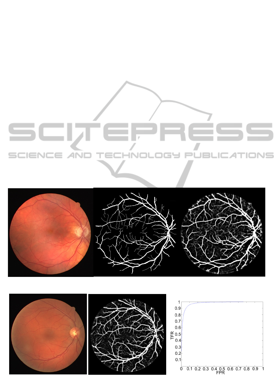
We tested our method on publicly-available
DRIVE dataset, which contains 40 images divided
into a test and training set, both containing 20 imag-
es. An example for an original image and manual
segmentation for the same image is shown in Figure
1. Note that picture that shows manual segmentation
is binary, but the output image is not, as outputs of
the DNN are probabilities of each pixel to be a blood
vessel. For practical purposes thresholding should be
done to obtain a binary image.
In the retinal vessel segmentation process, the
outcome is a pixel-based classification result. Notice
that we do not rely on any bottom-up segmentation,
since we treat semantic segmentation as pixel classi-
fication, where each pixel is described by its neigh-
borhood. Therefore the method is not affected by the
errors of bottom-up segmentation. In Figure 1 we
can see how a typical output image looks like. We
can see that areas belonging to blood vessels have
higher probability of being part of blood vessels.
In order to quantitatively measure the perfor-
mance of the proposed method we calculate the area
under the ROC curve for each image, accuracy, true
positive rate (TPR) and false positive rate (FPR).
TPR represents the fraction of pixels correctly de-
tected as vessel pixels while FPR is the fraction of
pixels erroneously detected as vessel pixels. The
accuracy is measured by the ratio of the total number
of correctly classified pixels to the number of pixels
in the image field of view. ROC curve plots the
fraction of TPR versus FPR.
The method achieves an average accuracy of
0.9466 with 0.7276 and 0.0215 TPR and FPR, re-
spectively on the DRIVE database. We obtained the
threshold using the optimal operating point on the
ROC curve, assuming the same costs of missclasify-
ing both classes.
Average AUC is 0.9749, where minimal AUC is
0.9665 and maximal 0.9843. The ROC curves are
calculated only for pixels inside the field of view of
the image. In Figure 2 and Figure 3 we can see the
original image, the softmax classification, and the
ROC curve for the given image. In Figure 2 AUC
reach maximum and in Figure 3 it is lowest. It can
be seen that in the figure with the lowest AUC seg-
mentation is much worse. That is due to pathologic
modifications (there are some exudates seen on the
original picture). In the DRIVE dataset there are not
many fundus images with pathologic changes and
Figure 1: Retinal images from DRIVE. From left to right: original image, manual segmentation and output image.
Figure 2: Original image, the softmax classification, and the ROC curve with maximum AUC (0.9843).
VISAPP2015-InternationalConferenceonComputerVisionTheoryandApplications
580
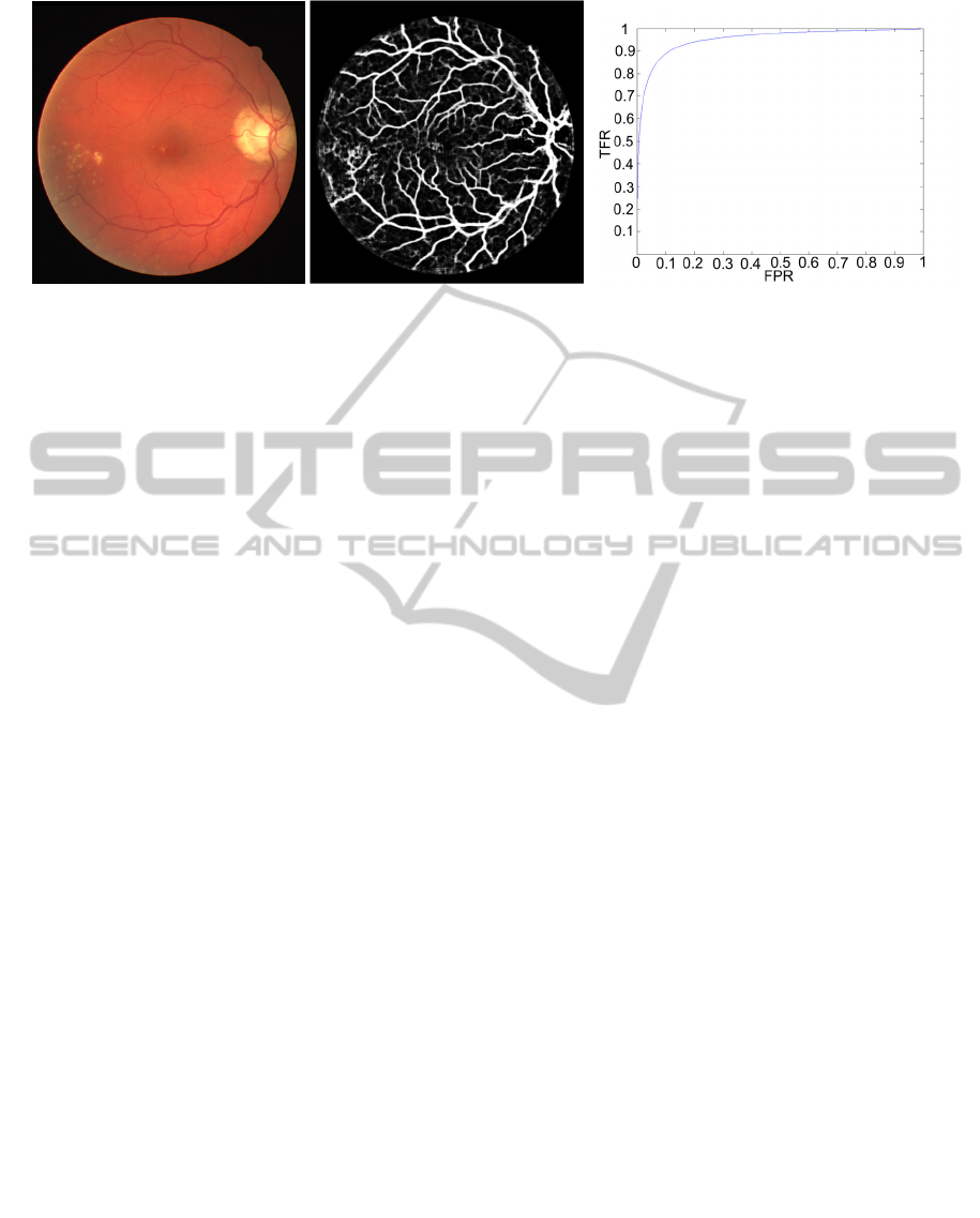
Figure 3: Original image, the softmax classification, and the ROC curve with lowest AUC (0.9665).
probably it would be possible to supress these false
positives by including more pathologies in the train-
ing, however that would require annotations for
pathologies and therefore such method would not be
comparable to the published work. We leave this
improvement for the future work.
5 CONCLUSIONS
The segmentation of the blood vessels in the retina
has been a heavily researched area in recent years.
Although many techniques and algorithms have
been developed, there is still room for further im-
provements.
We presented an approach using deep max-
pooling convolutional neural networks with GPU
implementation to segment blood vessels and results
show that it is promising method. Our method yields
the highest reported AUC for the DRIVE database,
to the best of our knowledge.
In Fraz et al. survey (2012) algorithms achieve
average accuracy in range of 0.8773 to 0.9597 and
AUC from 0.8984 to 0.961. Our method achieves an
average accuracy and AUC of 0.9466 and 0.9749,
respectively. Minimal AUC is 0.9665 and maximal
0.9843.
Future work would be to enhance the algorithm
by various methods like simulating more data for
training: using all channels (not only green), to ro-
tate, scale and mirror images etc. Perhaps some
preprocessing and postprocessing would enhance
results and surely averaging more networks would
improve results. Possibly foveation or non uniform
sampling is also a way to enhance results. Training
on a set with more images with pathologic changes
might improve results.
There is also room for experimenting with non-
linear activation functions to see whether they would
improve results.
ACKNOWLEDGEMENTS
Authors would like to thank Josip Krapac for help
with the definition and training of the neural net-
work.
REFERENCES
Abràmoff, M. D., Garvin, M. K., Sonka, M., 2010. Retinal
Imaging and Image Analysis. IEEE Rev. Biomed.
Eng. 3, 169–208. doi:10.1109/RBME.2010.2084567.
Bühler, K., Felkel, P., La Cruz, A., 2004. Geometric
methods for vessel visualization and quantification—a
survey. Springer.
Caffe | Deep Learning Framework [WWW Document],
n.d. URL http://caffe.berkeleyvision.org/ (accessed
10.2.14).
Cireşan, D.C., Giusti, A., Gambardella, L.M., Schmidhu-
ber, J., 2013. Mitosis detection in breast cancer histol-
ogy images with deep neural networks, in: Medical
Image Computing and Computer-Assisted Interven-
tion–MICCAI 2013. Springer, pp. 411–418.
Ciresan, D. C., Meier, U., Masci, J., Maria Gambardella,
L., Schmidhuber, J., 2011a. Flexible, high perfor-
mance convolutional neural networks for image classi-
fication, in: IJCAI Proceedings-International Joint
Conference on Artificial Intelligence. p. 1237.
Ciresan, D. C., Meier, U., Masci, J., Maria Gambardella,
L., Schmidhuber, J., 2011b. Flexible, high perfor-
mance convolutional neural networks for image classi-
fication, in: IJCAI Proceedings-International Joint
Conference on Artificial Intelligence. p. 1237.
Ciresan, D., Meier, U., Schmidhuber, J., 2012. Multi-
column deep neural networks for image classification,
in: Computer Vision and Pattern Recognition (CVPR),
2012 IEEE Conference on. IEEE, pp. 3642–3649.
Faust, O., Acharya, R., Ng, E.Y.-K., Ng, K.-H., Suri, J.S.,
2012. Algorithms for the automated detection of dia-
RetinalVesselSegmentationusingDeepNeuralNetworks
581

betic retinopathy using digital fundus images: a re-
view. J. Med. Syst. 36, 145–157.
Felkel, P., Wegenkittl, R., Kanitsar, A., 2001. Vessel
tracking in peripheral CTA datasets-an overview, in:
Computer Graphics, Spring Conference On, 2001.
IEEE, pp. 232–239.
Fraz, M. M., Remagnino, P., Hoppe, A., Uyyanonvara, B.,
Rudnicka, A. R., Owen, C. G., Barman, S. A., 2012.
Blood vessel segmentation methodologies in retinal
images – A survey. Comput. Methods Programs Bio-
med. 108, 407–433. doi:10.1016/j.cmpb.2012.03.009.
Fukushima, K., 1980. Neocognitron: A self-organizing
neural network model for a mechanism of pattern
recognition unaffected by shift in position. Biol. Cy-
bern. 36, 193–202.
Giusti, A., Caccia, C., Ciresari, D.C., Schmidhuber, J.,
Gambardella, L.M., 2014. A comparison of algorithms
and humans for mitosis detection, in: Biomedical Im-
aging (ISBI), 2014 IEEE 11th International Symposi-
um on. IEEE, pp. 1360–1363.
Image Sciences Institute: DRIVE: Digital Retinal Images
for Vessel Extraction [WWW Document], n.d. URL
http://www.isi.uu.nl/Research/Databases/DRIVE/ (ac-
cessed 10.2.14).
Kanski, J.J., Bowling, B., 2012. Synopsis of Clinical
Ophthalmology. Elsevier Health Sciences.
Kirbas, C., Quek, F., 2004. A review of vessel extraction
techniques and algorithms. ACM Comput. Surv.
CSUR 36, 81–121.
Lindeberg, T., 1998. Edge detection and ridge detection
with automatic scale selection. Int. J. Comput. Vis. 30,
117–156.
Magnier, B., Aberkane, A., Borianne, P., Montesinos, P.,
Jourdan, C., 2014. Multi-scale crest line extraction
based on half Gaussian Kernels, in: Acoustics, Speech
and Signal Processing (ICASSP), 2014 IEEE Interna-
tional Conference on. IEEE, pp. 5105–5109.
Masci, J., Giusti, A., Cireşan, D., Fricout, G., Schmidhu-
ber, J., 2013. A fast learning algorithm for image seg-
mentation with max-pooling convolutional networks.
ArXiv Prepr. ArXiv13021690.
Mitosis Detection in Breast Cancer Histological Images |
IPAL UMI CNRS - TRIBVN - Pitié-Salpêtrière Hos-
pital - The Ohio State University [WWW Document],
n.d. URL http://ipal.cnrs.fr/ICPR2012/ (accessed
10.17.14).
Niemeijer, M., Staal, J., van Ginneken, B., Loog, M.,
Abramoff, M.D., 2004. Comparative study of retinal
vessel segmentation methods on a new publicly avail-
able database, in: Medical Imaging 2004. pp. 648–656.
Patton, N., Aslam, T.M., MacGillivray, T., Deary, I.J.,
Dhillon, B., Eikelboom, R.H., Yogesan, K., Constable,
I.J., 2006. Retinal image analysis: Concepts, applica-
tions and potential. Prog. Retin. Eye Res. 25, 99–127.
doi:10.1016/j.preteyeres.2005.07.001.
Ricci, E., Perfetti, R., 2007. Retinal Blood Vessel Seg-
mentation Using Line Operators and Support Vector
Classification. IEEE Trans. Med. Imaging 26, 1357–
1365. doi:10.1109/TMI.2007.898551.
Schmidhuber, J., 2014. Deep Learning in Neural Net-
works: An Overview. ArXiv Prepr. ArXiv14047828.
Winder, R.J., Morrow, P.J., McRitchie, I.N., Bailie, J.R.,
Hart, P.M., 2009. Algorithms for digital image pro-
cessing in diabetic retinopathy. Comput. Med. Imag-
ing Graph. 33, 608–622.
VISAPP2015-InternationalConferenceonComputerVisionTheoryandApplications
582
