Pulse Reformation Algorithm for Leakage of Connected Operators
Gene Stoltz and Inger Fabris-Rotelli
Department of Statistics, University of Pretoria, Pretoria, South Africa
Keywords:
Discrete Pulse Transform, DPT, Leakage Problem, Pulse Reformation, Chaining.
Abstract:
The Discrete Pulse Transform (DPT) is a hierarchical decomposition of a signal in n-dimensions, built from
iteratively applying the LULU operators. The DPT is a fairly new mathematical framework with minimal
application and is prone to leakage within the domain, as are most other connected operators. Leakage is the
unwanted union of two connected sets and thus provides false connectedness information regarding the data.
The Pulse Reformation Framework (PRF) is developed to address the leakage problem within the DPT. It was
specifically tested with circular probes and showed successful object extraction of blood cells.
1 INTRODUCTION
The collection of LULU theory and the multiresolu-
tion analysis, namely the Discrete Pulse Transform
(DPT) was originally developed in (Rohwer, 2005)
for one dimension. The LULU operators and the DPT
were developed for multi-dimensions (Anguelov and
Fabris-Rotelli, 2010).
Within the DPT domain leakage occurs, as for
other connected operators. Leakage is the unwanted
union of arbitrary sets which heuristically should be
separate objects and is further developed theoretically
in Section 3. The leakage problem occurs when two
disconnected sets, after a certain operation on the
space these two sets become either connected as a by-
product of the operator, or the sets are connected due
to noise, low resolution and other such occurrences.
Leakage is also known as chaining (Soille, 2011).
According to (O’Callaghan and Bull, 2005) leakage
occurs due to the existence of weak points in the gra-
dient of object boundaries. Leakage is also inter-
preted as over segmentation. In (Li and Wilson, 1998)
the usage of multi-resolution techniques in conjunc-
tion with Markov random processes when doing tex-
ture segmentation to stop leakage is proposed. A pro-
posed solution to over-segmentation in segmentation
with partitioning of connected components based on
openings by treating all singletons generated by the
operator as elements from larger connected compo-
nents is discussed in (Ouzounis and Wilkinson, 2005).
The larger connected components refer to connectiv-
ity classes in higher dimensional space which are ex-
tensions of the normally defined connectivity classes
in mathematical morphology (Wilkinson, 2005).
Various other attempts has been made for cre-
ating solutions to the leakage problem, including
redefining existing connectivities (Goutsias et al.,
2000), (Tzafestas and Maragos, 2002), (Wilkinson,
2008)(Goutsias et al., 2000)(Tzafestas and Maragos,
2002) (Wilkinson, 2008). Another attempt at reduc-
ing leakage is the definition of stopping criteria in
morphological opening and opening by reconstruc-
tion (Terol-Villalobos et al., 2006). Serra also sug-
gested the idea of using a circular structuring element
to refine connectivity in order to deal with leakage
(Serra, 2005).Leakage exists in other image process-
ing spaces such as the active-contour model where
possible reduction in leakage is to estimate the po-
sition of possible edges in the image by minimal
weighted local variance (Law and Chung, 2006). Gra-
ham et al (Graham et al., 2008) used adaptive param-
eters within the active-contour model to possibly stop
estimated leakage.
We propose a framework called Pulse Reforma-
tion Framework (PRF) to resolve leakage within the
DPT domain. The framework is developed for two
dimensional data which includes any type of image
in the conventional sense. We use circular probes to
resolve leakage in the domain, however alternatives
are easily interchangeable. The framework is applied
to a small set of blood cells. On basis of the PRF
within the LULU scale-space a spot detector is devel-
oped and compared.
583
Stoltz G. and Fabris-Rotelli I..
Pulse Reformation Algorithm for Leakage of Connected Operators.
DOI: 10.5220/0005313205830590
In Proceedings of the 10th International Conference on Computer Vision Theory and Applications (VISAPP-2015), pages 583-590
ISBN: 978-989-758-089-5
Copyright
c
 2015 SCITEPRESS (Science and Technology Publications, Lda.)

2 THE DISCRETE PULSE
TRANSFORM
An n-monotone sequence is part of a connectivity
class and is thus a connected set. The concept of an n-
monotone sequence is extended to higher dimensions
with the introduction of connectivity classes (Serra,
1982).
Definition 2.1. Let E be an arbitrary nonempty set.
A family C ∈ P (E) is called a connectivity class if
the following axioms hold: (1.)
/
0 ∈ C (2.) {x
i
} ∈ C
for every i such that x
i
∈ E (3.) For each C
j
∈ C and
T
j∈I
C
j
6=
/
0, then
S
j∈I
C
i
∈ C .
Any element of C is called a connected set. We
can now extend to d-dimensions such that x ∈ Z
d
,d ∈
N so that the LULU operators operate on n-connected
sets in d-dimensions but with a discrete space is suf-
ficiently rich in connected sets. The required condi-
tions for such a rich connectivity space is found in
(Anguelov and Fabris-Rotelli, 2010).
For any set of cardinality n + 1 we can now de-
fine within the d-dimensional space connected sets
which contain the point x ∈ Z
d
, N
n
(x) = {V ∈ C : x ∈
V,card(V ) = n+1}. The LULU operators defined on
an Abelian group A(Z
d
) such that commutativity al-
ways holds within the lattice, are as follows:
Definition 2.2. Let f ∈ A(Z
d
) and n ∈ N. Then for
x ∈ Z
d
: L
n
( f )(x) = max
V ∈N
n
(x)
min
y∈V
f (y) and
U
n
( f )(x) = min
V ∈N
n
(x)
max
y∈V
f (y).
The operators defined in Definition 2.2 operate
only on local maximum sets and minimum sets in the
space. With the concept of adjacency we can classify
a connected set as a local minimum or a local maxi-
mum.
Definition 2.3. Let V ∈ C and f ∈ A(Z
d
) then V is
called a local maximum (minimum) set if:
max(min)
y∈adj(V )
{ f (y)} < (>)min(max)
x∈V
{ f (x)},
where adj(V ) = {x ∈ Z
d
: x 6∈ V,V ∪ {x} ∈ C }.
The L
n
operator removes local maximums of size
smaller and equal to n while U
n
removes local mini-
mums of size smaller or equal to n. The two operators
can’t create new local maximum sets or minimum sets
but they may enlarge the cardinality of a connected
set attributed to it. The LULU operators maintain
their properties from the one dimensional theory such
as being a separator, being fully trend preserving and
preserving total variation, as well as all other proper-
ties. The DPT in multi-dimensions is represented as
DPT ( f ) = [D
1
( f ), D
2
( f ), ..., D
N−1
( f )]. Each compo-
nent D
n
is calculated as
D
1
( f ) = (I − P
1
)( f )
D
n
( f ) = (I − P
n
) ◦ Q
n−1
( f ), n = 2, ..., N − 1
where P
n
= L
n
◦U
n
or P
n
= U
n
◦ L
n
and Q
n
= P
n
◦ ... ◦
P
1
,n ∈ N.
Definition 2.4. A function ψ ∈ A(Z
d
) is called a
pulse if there exists a connected set V and a nonzero
real number α such that
ψ(x) =
(
α, i f x ∈ V
0, i f x ∈ Z
d
\V.
Each different scale D
n
is then D
n
( f ) =
∑
γ(n)
s=1
ψ
ns
and
f =
N−1
∑
n=1
γ(n)
∑
s=1
ψ
ns
where γ(n) is the total number of local maximum and
local minima of size n and ψ is a pulse (def 2.4).
The DPT decomposition forms a scale-space for-
mally defined in: (Fabris-Rotelli, 2012):
Definition 2.5. Let f ∈ A(Z
d
). The set S
f ,Λ
=
{(λ,L
f
(λ)) : λ ∈ Λ} is called a scale-space of f gener-
ated by the operator L with respect to scale parameter
set Λ and measure of smoothness S ∈ A(Z
d
).
S is a function called the measure of smoothness
which is dependant on the requirement of the specific
task. Overall a very smooth signal yields a smooth-
ness measure of 0 where rougher signals yield higher
values. In the case of the DPT the measure of smooth-
ness determines how close the current sequence is
to its local monotonicity (Fabris-Rotelli, 2012). The
interested reader can find more information in Dis-
crete Pulse Transform of images and applications
(Fabris-Rotelli, 2012). Some relations with mathe-
matical morphology are however obvious. Firstly the
LULU smoothers are exactly the area opening and
closing operators (Vincent, 1193), but were devel-
oped independently from the one-dimensional LULU
smoothers (Rohwer, 2005; Rohwer and Laurie, 2006;
Rohwer and Toerien, 1991). They can thus be com-
pared to a morphological pyramid (Salembier and
Serra, 1995; Morales et al., 1995), but are however
valid in N dimensions and do not require the restric-
tion of a predetermined structuring element. The DPT
does replicate the nice property of a morphological
pyramid of nested flat zones, allowing for image sim-
plification while preserving contour information.
The DPT forms the scale-space S
f ,LU LU
=
{(n,P
n
( f )) : n ∈ Λ
0
= {0,1,2,...,N}} called the
LULU scale-space. A scale-space allows the tracking
of structures within a domain through different scales
ranging from fine to coarse.
VISAPP2015-InternationalConferenceonComputerVisionTheoryandApplications
584

3 LEAKAGE
We provide a formal definition for leakage as:
Definition 3.1. Let Φ : Z
d
→ Z
d
be an arbitrary op-
erator. If there exists

X
i
⊂ Z
d
,i ∈ I,X
i
∈ C

with
∩
i∈I
X
i
=
/
0 such that ∪
i∈I
Φ(X
i
) ∈ C then Φ is said
to have caused leakage.
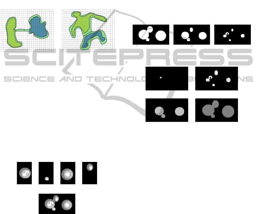
An operator Φ may satisfy Definition 3.1 in dif-
ferent mannerisms. Consider Figure 1, an example of
desired and undesired leakage.
X
1
X
2
Φ(X
1
)
Φ(X
2
)
(a)
X
1
X
2
Φ(X
1
)
Φ(X
2
)
(b)
Figure 1: (a) Undesired Leakage, (b) Desired leakage.
In Figure 1(a), after applying operator Φ, the leak-
age formed is undesired. Object Φ(X
1
) and Φ(X
2
)
should be separate objects. However, in Figure 1(b)
object X
1
and X
2
should be one. After applying the
operator to the image the two objects get connected as
desired. Leakage are generally dealt with by directly
applying a problem specific solution. TO distinguish
between different kinds of leakage we define a mea-
sure of observed leakage as follows:
Definition 3.2. The strength of a leakage is measured
as 1/card(A
Strength
) where A
Strength
= {{x
i
,x
j
} ∈ C :
x
i
∈ Φ(X
i
),x
j
∈ Φ(X
j
),i 6= j,i, j ∈ I}.
(a) (b) (c) (d)
(e) Combined ob-
jects
Figure 2: Synthetic Objects in an image.
The larger the strength of the leakage the larger
the undesired effect is on the image. It is clear then
in the case of a good smoother desired leakage will
occur.
A synthetic example is created to demonstrate the
leakage problem. Four objects with varying internal
intensities shown in Figure 2 are combine into a sin-
gle image. The four objects need to be extracted.
To extract the different objects we can use connected
components to indicate individual objects. A set con-
sisting of connected components will then denote one
object. Two simplistic methods can be used. The first
is the use of thresholding. The synthetic image can
be thresholded at three different levels as the image
only consists of four discrete grey levels. The thresh-
olded images are shown in Figure 3. In Figure 3 it
is clear that no threshold will yield 4 connected sets
which will cohere with the four original objects. An-
other way, is to use the DPT scale-space and threshold
different pulse sizes. We choose four different pulse
ranges which are shown in Figure 4.
(a) (b) (c)
Figure 3: Synthetic image thresholded at 3 different levels.
(a) n ∈ [0, 400) (b) n ∈ [400, 3600)
(c) n ∈ [3600, 6400) (d) n ∈ [6400, 21800)
Figure 4: Synthetic images thresholded for different pulse
ranges.
Even using the DPT scale-space it is not possi-
ble to extract four connected components that will
yield the required connected sets. In Figure 3 and 4
leakage is evident in most of the thresholded images.
Although technically there exist many other ways to
possibly extract the objects, this problem was only
used to illustrate leakage in simple connected compo-
nents and DPT framework. In the next section we de-
scribe a proposed method to eliminate leakage within
the DPT framework.
4 THE PULSE REFORMATION
FRAMEWORK (PRF)
To explain the proposed framework one can visual-
ize the leakage problem as a box of brittle magnets.
The task is to successfully remove all the magnets
from the box and place the individual ones in a row.
The problem lies in identifying these individual mag-
nets. Two or more magnets can be stuck together and
PulseReformationAlgorithmforLeakageofConnectedOperators
585

must be pulled apart. However an individual magnet
can only be separated from itself by breaking it. By
looking at structural cues we can separate these mag-
nets, such as if two balls are stuck together they most
probably must be separated. If two cubes, unaligned,
are stuck together we can assume they must be sep-
arate. If a sphere and a pyramid are stuck together
they must probably be separated. We can thus con-
tinue like this for all kinds of known shapes and say
with high probability that these different structures do
not fit together.
ψ
ms
1
→ R
ms
1
R
ns
23
ψ
ns
2
=
3
S
i=1
R
ns
2i
R
ns
21
R
ns
22
Figure 5: A DPT pulses stacked in different scale.
The scales from the DPT can be stacked from the
smallest to the largest scale forming the LULU scale-
space. A visual demonstration is shown in Figure 5.
The pulses in Figure 5 are said to form a stack de-
fined by the scale-space neighbourhood relation given
below in Definition 4.1 and Definition 4.2.
Definition 4.1. Two arbitrary DPT pulses, ψ
ns
2
and
ψ
ms
1
with n < m, are called scale-space neighbours if
ψ
ns
2
⊂ ψ
ms
1
and for any other DPT pulse ψ
ps
3
,
n < p < m we have ψ
ps
3
∩ ψ
ns
2
=
/
0.
The strength of the scale-space neighbour relation
is measured as the inverse of the difference in cardi-
nality of the two pulses φ
ns
2
and φ
ms
1
, naturally
1
m−n
.
Definition 4.2. A collection of DPT pulses are said to
form a stack if they are each scale-space neighbours
of at least one other pulse in the collection.
In Figure 5 the pulses illustrated form a stack. The
PRF algorithm will obtain the true pulses R
ns
21
, R
ns
22
and R
ns
23
.
By using Definition 4.2 we can say that every
pulse consists of regions so that ψ
ns
=
p
S
i=1
R
ns
k
. This
is demonstrated in Figure 6. Assume that Figure 6 is
an image of two separate balls, thus two individual
objects. Inspecting Figure 6, only one object is ob-
served, the full pulse ψ
ns
2
. The two objects are linked
by a third region. The third object is then referred to
as a leakage region, which on its own can possibly
also be an object or noise. If we want to eliminate
leakage we need to estimate the true regions R
ns
21
,
R
ns
22
and R
ns
23
.
Leakage
ψ
ns
2
=
3
S
i=1
R
ns
2i
R
ns
21
R
ns
22
R
ns
23
Figure 6: A pulse extracted by the DPT showing the possi-
ble regions which the pulse consists of.
We aim to, in the LULU scale-space, objectively
eliminate leakage. In case of the magnet box we aim
at finding all the rigid shapes with the most probable
shape having the least amount of edges. We can then
objectively eliminate leakage.
The proposed framework will be developed us-
ing circular probes. Other shapes can also be used
within the framework. Using the PRF, circular ob-
ject within the LULU scale-space will produce strong
joined stacks. A joined stack is formed when a group
of scale-space neighbours forming a stack also cohere
to an additional requirement. The additional require-
ment involves a principle point
˜
R
ns
k
for each region
R
ns
k
. The principle point needs to capture the core
structure of the region. The principle point of circular
object is at the arithmetic mean in terms of the spatial
domain, is always surrounded by edges and the point
lies within the object. It can be assumed that the cen-
tre of a circle will capture the core purpose of circular
objects. The circular object can also be reconstructed
from the principle point by iteratively increasing the
radius of the circle centred at the principle point. In
general if using any shaped probe, the principle point
˜
R
ns
k
should be scale invariant, translation invariant,
rotation invariant, and affine invariant.
In Figure 7 the red dot shows the principle point
and the dark blue shows elements part of the geomet-
rical set. The principle point of the doughnut shape in
Figure 7 can be defined as the centre of a circle which
is not contained within the set but is surrounded by
a continuous edge. The principle point of a concave
mirror shape should lie at the focal point of the con-
cave side of the set. The principle point of a triangle
should lie in the middle of the shortest edge. From
all of these principle points the objects can be recon-
structed by knowing one extra parameter such as the
radius or distance of a corner or edge in the set. To es-
timate a region’s principle point, we iteratively erode
the pulse until the next erosion yields an empty set.
VISAPP2015-InternationalConferenceonComputerVisionTheoryandApplications
586

Figure 8 illustrates this. The last non-empty erosions
will represent the principle points of the regions and
also indicated the number of regions the pulse is made
up of. The regions can then be reconstructed by dilat-
ing each principle point until the defined energy func-
tion E
ns
below is minimized over every region of the
pulse simultaneously.
Figure 7: Examples of possible principle points denoted by
the red dot.
Original
After 1st erosion
After 2nd erosion
After 3rd erosion
After 4th erosion
ψ
ns
˜
R
ns
2
˜
R
ns
1
Figure 8: Example of finding the principle points in a pulse.
Each region R
ns
k
will have a principle point, thus
each pulse can contain multiple principle points. The
regions must adhere to the boundary conditions of the
DPT scale-space thus
R
ns
k
=

R
ns
k
∩ ψ
ns

/
[
k6=i
(R
ns
i
). (1)
The regions within a pulse can only consist of
unique elements thus every element in a pulse can
only be assigned to one region. From the principle
point each region is reconstructed by minimizing the
energy function E
ns
. For the circular probes we can
define an energy function
E
ns
=
p
∑
k=1
κ(s
k
)
∑
t=1
card{ζ(t − 1,
˜
R
ns
k
)}
|card{ζ(t,
˜
R
ns
k
)} − card{ζ(t − 1,
˜
R
ns
k
)}|
where ζ(t,
˜
R
ns
k
) denotes a set containing all the ele-
ments within a circle of radius t centred at
˜
R
ns
k
, the
t
th
dilation of the circular set centred at the princi-
ple point, while staying within the boundary of the
pulse; where p is the number of regions; and κ(s
k
)
the appropriate t number of dilations where t is a ge-
ometrical parameter. The energy function determines
the best circles centred at the principle points asso-
ciating each pulse element to a region, restricted to
the boundary conditions in equation 1. The created
regions and found principle point can be compared
techniques such as the medial axis transform and the
resulting skeleton by maximal balls (LVincent and
Dougherty, 1994).
Next we need to relate regions at different scales
to one another. Each region has the apparent same
defining principle point which should then be posi-
tioned at a known position between scales. Specif-
ically for circular objects all the principle points
should be at the same geometrical position. We can
thus say that two or more regions form a joined stack
(Definition 4.4) if the principle point(s) are joined
(Definition 4.3) and the regions form a stack (Defi-
nition 4.2).
Definition 4.3. Two scale-space neighbours ψ
ns
and
ψ
ms
with n < m containing regions R
ns
j
and R
ms
i
with geometrical parameters r
j
, r
i
and principle points
˜
R
ns
j
,
˜
R
ms
i
, are said to have joined principle points if
J(
˜
R
ns
j
,
˜
R
ms
i
) < ε = N (
˜
R
ns
j
,
˜
R
ms
i
,r
i
,r
j
) where J is the
joining function and N is a noise function.
The joining function J provides a relation between
of the two principle points and can be any type of
polygon or line. The noise function N provides a
measure of how similar the two regions are based on
the expected relative position of the principle points.
For the circular case we define r
j
= κ(s
j
), r
i
= κ(s
i
)
and J(
˜
R
ns
j
,
˜
R
ms
i
) = k
˜
R
ns
j
,
˜
R
ms
i
k with k·, ·k giving the
euclidean distance between the two points. We also
define our noise function N (
˜
R
ns
j
,
˜
R
ms
i
,κ(s
i
),κ(s
j
))
= (card{R
ns
i
}/card{R
ms
j
}) ∗ (κ(s
i
)/κ(s
j
)).
Definition 4.4. Two regions R
ns
j
and R
ms
i
with n < m
form a joined stack if their principle points are joined
and R
ns
j
⊆ R
ms
i
.
This definition is visually shown in Figure 9 where
J(
˜
R
ns
j
,
˜
R
ms
i
) = a. The ε can be interpreted as a
noise canceller within the LULU scale-space. If
a perfect scale-space was constructed all the pulses
forming joinings belong to the same object and will
have aligned principle points. In Figure 9 the large
coloured dots denote the principle point in each re-
gion.
r
i
R
ms
i
R
ns
j
r
j
a
a
Figure 9: The joining of two arbitrary pulses.
The strength of the joining of the two regions can
be measured as the strength of a scale-space neigh-
bour. The smaller the difference in cardinality of the
two regions, the stronger the joining becomes. An
additional strength measure can be added such as the
variation of the principle points from the expected dis-
tance.
PulseReformationAlgorithmforLeakageofConnectedOperators
587

We have now shown that we can estimate regions
from pulses. We estimate a region from the first es-
timated principle point and then re-estimate the prin-
ciple point using the region. This process can be re-
peated until the principle point moves less than the
noise function N and E
ns
is minimized.
The estimation of the regions within pulses can be
represented by a four corner model. The four nodes
are the Principle Point node, the Pulse node, the Join-
ing node and the Regions node. The nodes are shown
in Figure 10(a). Each node’s name is self-evident of
the represented data at the node. The arrows present
the process that needs to be executed to transform one
set of data to another.
(a) (b)
Figure 10: (a) Region based Pulse Reformation Model. (b)
Region based Pulse Reformation Model.
The Pulse node can be used to estimate the Prin-
ciple Points node. The Principle Points node is used
to estimate the Regions and to determine joining with
other scale-space neighbour regions. The Joining
node can be used to estimate the Regions node. The
Regions node can estimate the Principle Points as
well as the Pulse node. This whole process follows
an iterative nature.
To create a more robust estimation of the regions
we need to estimate each region by including the
structure of the complete LULU scale-space. The
PRF uses an iterative approach to first estimate an
initial principle point which is used to estimate the
regions within each pulse. The principle points that
form a joined stack can be used to adjust principle
points and re-estimate the regions until all energy
functions E
ns
and all joining functions J(·) have been
minimized. This combined iterative model is repre-
sented in Figure 10(b).
After the PRF has been applied the LULU
scale-space consists of various joined stacks.
Each joined stack will have a joined stack
strength which is calculated by the sum of the
strength of the scale-space neighbours within the
joined stack divided by the number of regions con-
tained in the joined stack. The strongest joined stacks
will then present the most salient objects.
To be able to use the PRF four main things need
to be defined: (1.) The Principle Point Estimator
˜
R
ns
k
.
(2.) The Energy function E
ns
which needs to be mini-
mized. (3.) The joining function J(·). (4.) The noise
function or principle point alignment ε. Each of these
functions have already been defined for the case of
circular objects.
5 SYNTHETIC LEAKAGE
REDUCTION
We can now apply the PRF to the synthetic image
created in Figure 2. In Figure 11 the output of the
framework is shown. Four different objects were ex-
tracted each coinciding with a synthetic object. Each
extracted object shows protrusion where leakage oc-
curred. This is where the framework has an uncer-
tainty as to which principle point the region elements
belong.
(a) (b)
(c) (d)
Figure 11: The Pulse Reformation of the synthetic image.
The extracted objects can easily be thresholded
just above zero to provide four discrete connected sets
which then coincide with the original objects. The
PRF can now be tested on a real world image. An-
other example application appears in (Fabris-Rotelli
and Stoltz, 2012).
6 SPOT DETECTION
The PRF can be used for spot detection. We can
not only extract the strongest joined stacks but only
the joined stack who’s bottom region or top region is
within a certain range. For spot detection the bottom
region of the joined stack must be smaller or equal to
the largest expected spot.
Fixed cell imaging of individual mRNA molecules
is accomplished by using 48 or more singly labelled
oligonucleotide probes (Raj et al., 2008). By utilizing
fluorescent microscopy the mRNA becomes compu-
tationally identifiable fluorescent spots. There can be
hundreds of mRNA in a cell. An effective spot detec-
tor and spot counter is thus required.
VISAPP2015-InternationalConferenceonComputerVisionTheoryandApplications
588

A current spot detector exists which uses thresh-
olding of a difference of two Gaussians (Raj et al.,
2008). The DoG spot detector has three different pa-
rameters which can be modified: the range of the
Gaussian window, the variance of the Gaussian and
the specific threshold. In depth the method actually
has 5 parameters as both the Gaussians must be se-
lected, each with a window and a variance. Usually
one Gaussian is assumed to be the original image.
Our spot detector will only use the joined stacks
with a bottom pulse cardinality smaller than a set
size. These joined stacks are then thresholded by the
joined stack strength to remove the very weak joined
stacks. The PRF spot detector then only uses 2 param-
eters: the expected size of the objects and the thresh-
old value.
For the experiment we created our own ground
truth. The ground truth was not evaluated by an expert
in mRNA thus we can not measure the algorithms true
performance but only the relative performance. The
DoG spot detector was confirmed to be an accurate
detector but was not quantified (Raj et al., 2008). The
two test images and their ground truths are shown in
Figure 12.
(a) (b)
(c) Images of mRNA
(Raj et al., 2008)
(d) Ground truths
Figure 12: Fluorescent microscopy images of mRNA.
The two algorithms will be evaluated by using
precision-recall graphs (Powers, 2011). The preci-
sion (t p/(t p + f p)) and recall (t p/(t p + f n)) is used
to calculate the f -measure:
F-measure = 2 ·
Precision · Recall
Precision + Recall
.
The true positives, t p, are measured by taking the
number of correctly detected spots thus the detected
spots that coincide with the ground truth. The false
positives, f p, are measured by all the spots that do
not coincide with ground truth. If two spots are de-
tected close together and both coincide with one spot
on the ground truth, one is taken as correct and the
other is then a false positive. The false negatives, f n,
are calculated as all the spots in the ground truth that
were not detected by the spot detection algorithm.
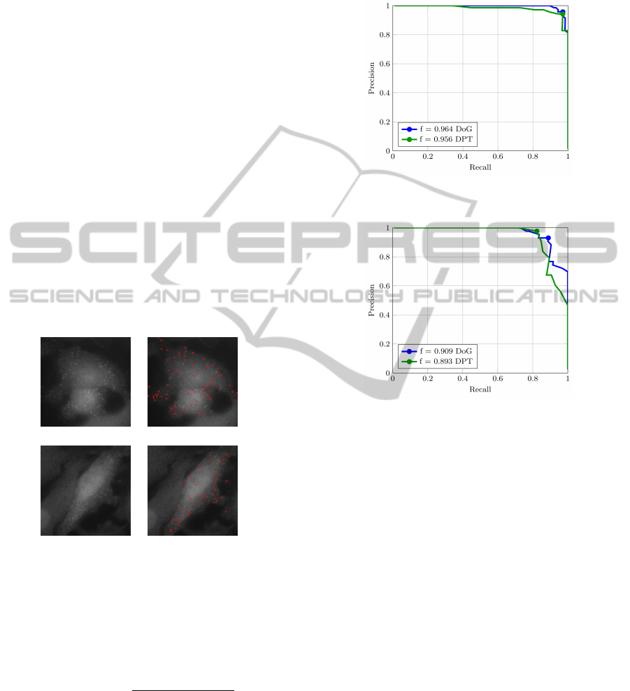
Figure 13: The first Precision-Recall graph for the DPT and
DoG spot detectors.
Figure 14: The second Precision-Recall graph for the DPT
and DoG spot detectors.
In Figures 13 and 14 the f -measures are plot-
ted for increasing threshold values. The maximum
f -measures are indicated on the graphs.
Both the algorithms perform well. The PRF spot
detector using the DPT is 1% less accurate than the
DoG method. Taking into account that the DPT
method has 3 less parameters to tune than the DoG
method and is less sensitive to its parameters the DPT
method is superior to the DoG method. The sensitiv-
ity of the DoG method to the chosen variance param-
eter is high as the chosen variance propagates to each
pixel in the image. Choosing the correct variance for
a Gaussian function is also not a trivial matter. The
DPT method is not very sensitive to the expected size
of the spot as long as the expected size is greater than
the actual size of the spot. The expected size of the
spot is easily measured by looking at the number of
pixels within the spot.
7 CONCLUSION
We have provided a theoretical settings for leakage
PulseReformationAlgorithmforLeakageofConnectedOperators
589

within the DPT as well as an effective algorithm to
deal with leakage in images and have applied the tech-
nique to salient object detection and a more specific
application in spot detection within the DPT frame-
work. Future work will look at developing a non-
shape dependent reformation algorithm taking advan-
tage of the non-shape dependent nature of the DPT.
In addition, relaxing the pulse definition to allow for
quasi-flat connected components (Soille, 2011) may
add to a more efficient DPT as well as a more robust
reformation algorithm.
ACKNOWLEDGEMENTS
The authors acknowledge funding received from the
NRF Competitive Support for Unrated Researchers
CSUR13082931658.
REFERENCES
Anguelov, R. and Fabris-Rotelli, I. (2010). LULU oper-
ators and Discrete Pulse Transform for multidimen-
sional arrays. Image Processing, IEEE Transactions
on, 19(11):3012–3023.
Fabris-Rotelli, I. and Stoltz, G. (2012). On the leakage
problem with the Discrete Pulse Transform decompo-
sition. In de Waal, A., editor, Proceedings of the 23rd
Annual Symposium of the Pattern Recognition Associ-
ation of South Africa, pages 179–186.
Fabris-Rotelli, I. N. (2012). Discrete Pulse Transform of
images and applications. PhD thesis, University of
Pretoria.
Goutsias, J., Vincent, L., and Bloomberg, D. S. (2000).
Mathematical morphology and its applications to im-
age and signal processing, volume 18, chapter Practi-
cal extensions of connected operators, pages 97–110.
Springer.
Graham, M. W., Gibbs, J. D., and Higgins, W. E. (2008).
Robust system for human airway-tree segmentation.
In Medical Imaging, pages 69141J–69141J. Interna-
tional Society for Optics and Photonics.
Law, W. and Chung, A. C. (2006). Minimal weighted lo-
cal variance as edge detector for active contour mod-
els. In Computer Vision–ACCV 2006, pages 622–632.
Springer.
Li, C.-T. and Wilson, R. (1998). Image segmentation based
on a multiresolution bayesian framework. In Image
Processing, 1998. ICIP 98. Proceedings. 1998 Inter-
national Conference on, pages 761–765. IEEE.
LVincent and Dougherty, E. (1994). Digital Image Process-
ing Methods, chapter Morphological segmentaion fro
textures and particles, page Chapter 2. Marcel Dekker,
Inc.
Morales, A., Acharya, R., and Ko, A.-J. (1995). Morpho-
logical pyramids with alternating sequential filters.
IEEE Transactions on Image Processing, 4(7):965–
977.
O’Callaghan, R. J. and Bull, D. R. (2005). Combined
morphological-spectral unsupervised image segmen-
tation. Image Processing, IEEE Transactions on,
14(1):49–62.
Ouzounis, G. K. and Wilkinson, M. H. (2005). Countering
oversegmentation in partitioning-based connectivities.
In Image Processing, 2005. ICIP 2005. IEEE Interna-
tional Conference on, volume 3, pages III–844. IEEE.
Powers, D. M. (2011). Evaluation: from precision, recall
and f-measure to roc, informedness, markedness &
correlation. Journal of Machine Learning Technolo-
gies, 2(1):37–63.
Raj, A., van den Bogaard, P., Rifkin, S. A., van Oudenaar-
den, A., and Tyagi, S. (2008). Imaging individual
mrna molecules using multiple singly labeled probes.
Nature methods, 5(10):877–879.
Rohwer, C. (2005). Nonlinear Smoothers and Multiresolu-
tion Analysis. Birkhauser.
Rohwer, C. and Laurie, D. (2006). The Discrete Pulse
Transform. SIAM journal on mathematical analysis,
38(3):1012–1034.
Rohwer, C. and Toerien, L. (1991). Locally monotone ro-
bust approximation of sequences. Journal of compu-
tational and applied mathematics, 36(3):399–408.
Salembier, P. and Serra, J. (1995). Flat zones filtering, con-
nected operators, and filters by reconstruction. IEEE
Transactions on Im, 4(8):1153 – 1160.
Serra, J. (1982). Image Analysis and Mathematical Mor-
phology. Vol I, and Image Analysis and Mathematical
Morphology. Vol II: Theoretical Advances. Academic
Press, London.
Serra, J. (2005). Viscous lattices. Journal of Mathematical
Imagin, 22:269–282.
Soille, P. (2011). Preventing chaining through transitions
while favouring it within homogeneous regions. In
Soille, P., Pesaresi, M., and Ouzounis, G., editors,
Mathematical Morphology and Its Applications to Im-
age and Signal Processing, volume 6671 of Lecture
Notes in Computer Science, pages 96–107. Springer
Berlin Heidelberg.
Terol-Villalobos, I. R., Mendiola-Santib
´
a
˜
nez, J. D., and
Canchola-Magdaleno, S. L. (2006). Image segmen-
tation and filtering based on transformations with re-
construction criteria. Journal of Visual Communica-
tion and Image Representation, 17(1):107–130.
Tzafestas, C. S. and Maragos, P. (2002). Shape connectiv-
ity: multiscale analysis and application to generalized
granulometries. Journal of Mathematical Imaging and
Vision, 17(2):109–129.
Vincent, L. (1193). Grayscale area opening and closings,
their efficient implementation and applications. In
Proceedings of the EURASIP Workshop on Mathemat-
ical Morphology and its Applications to Signal Pro-
cessing, Barcelona, Spain.
Wilkinson, M. (2005). Attribute-space connected filters.
In Ronse, C., Najman, L., and Decencire, E., editors,
Mathematical Morphology: 40 Years On, volume 30
of Computational Imaging and Vision, pages 85–94.
Springer Netherlands.
Wilkinson, M. H. (2008). Connected filtering by recon-
struction: Basis and new advances. In Image Process-
ing, 2008. ICIP 2008. 15th IEEE International Con-
ference on, pages 2180–2183. IEEE.
VISAPP2015-InternationalConferenceonComputerVisionTheoryandApplications
590