Mesh Alignment using Grid based PCA

David Kaye and Ioannis Ivrissimtzis

School of Engineering and Computing Sciences, Durham University, Durham, U.K.

Keywords:

Mesh Alignment, Principal Component Analysis, Grid Based Methods.

Abstract:

We present an algorithm for mesh alignment by performing Principal Components Analysis (PCA) on a set

of nodes of a regular 3D grid. The use of a 3D lattice external to both inputs increases the robustness of

PCA, particularly when dealing with meshes of different and possibly uneven vertex density. The proposed

algorithm was tested on meshes that have undergone standard mesh processing operations such as smooth-

ing, simpliﬁcation and remeshing. In several cases the results indicate an improved robustness compared to

performing PCA directly on mesh vertices.

1 INTRODUCTION

It is often useful to compare two meshes, point clouds,

or a mixture of the two. For example, in shape recog-

nition one might compare two meshes or two point

clouds asking whether they belong to the same cate-

gory.

The comparison of two meshes usually starts with

their alignment. It should be noted that the exact way

in which two meshes are best aligned is not clearly de-

ﬁned. In fact, the best alignment can be application-

dependent, and mesh alignment should be seen as an

ill-posed problem. Nevertheless, a good alignment al-

gorithm is expected to be able to align a mesh with a

version of it that has undergone common mesh pro-

cessing operations such as smoothing, simpliﬁcation

or remeshing.

Alignment is typically done by computing a trans-

lation, a scaling and a rotation, which are then ap-

plied to one of the meshes to align it with the other.

The computation of the translation is usually done

by aligning barycentres, while the scaling is done by

aligning bounding boxes or bounding spheres (Sﬁkas

et al., 2014). Translation and scaling are both con-

sidered less challenging to compute than the rota-

tion, which is the focus of this paper. In some ﬁelds

such as medical imaging, the registration process re-

quires more than this simple pose normalisation, for

instance, an alignment between certain parts of the

two models (Postelnicu et al., 2009).

The simplest and most widely used method for the

rotational alignment of two meshes aligns the princi-

pal axes of the mesh vertex sets. Despite its popu-

larity, it is well documented that in demanding appli-

cations such as shape recognition the results of this

alignment method may not be satisfactory, especially

in the case when the mesh undergoes processing that

potentially disturbs the distribution of mesh vertices

such as simpliﬁcation and remeshing.

One way around this problem is to voxelise the

mesh and then apply an alignment algorithm for vol-

umetric data. However, such a method can be compu-

tationally demanding, and the cost of the voxelisation

cannot be fully justiﬁed if it is used for mesh align-

ment only. A second approach would be to apply PCA

not on the mesh vertex set but on a more uniform point

set produced by a mesh sampling method. However,

such a method would depend on the quality of the tri-

angulation and for example, a large number of long

thin triangles in the mesh could cause problems.

Here, we propose a solution in between the above

two approaches, that is, a sampling method which,

without being a fully volumetric method, is based on

creating a subset of the nodes of a regular grid and

then performing PCA on that point set.

1.1 Contribution

We present a deterministic, fully automatic method

for mesh alignment based on performing PCA on a

point sample on a regular grid. The algorithm can also

process point clouds as inputs, allowing point clouds

to be aligned with meshes, or two point clouds to be

aligned. However, when connectivity exists, it is used

to increase the robustness of the usual PCA on the

mesh vertex set, which can be problematic when, for

instance, the mesh vertex set is very sparse.

174

Kaye D. and Ivrissimtzis I..

Mesh Alignment using Grid based PCA.

DOI: 10.5220/0005313801740181

In Proceedings of the 10th International Conference on Computer Graphics Theory and Applications (GRAPP-2015), pages 174-181

ISBN: 978-989-758-087-1

 2015 SCITEPRESS (Science and Technology Publications, Lda.)

1.2 Limitations

The main limitation of the algorithm is that since PCA

is applied to a subset of the nodes of a relatively

coarse grid, the method is less accurate than the usual

PCA on mesh vertices when the two meshes are iden-

tical or almost identical. In a sense, this larger error

is a trade-off for the increased robustness and our ex-

periments show that it is in a range that in most appli-

cations would be considered tolerable.

Since the method is underpinned by PCA, it is not

particularly well suited for inputs that have high levels

of rotational symmetry. Finally, since the algorithm is

highly geometric in nature, it could be challenging to

adapt to incorporate non-geometric primitives such as

colour (Roy et al., 2004).

2 RELATED WORK

Most of the work on mesh alignment focuses on and

enhances the Iterative Closest Point (ICP) algorithm,

which takes a set of points common to both input

meshes and iteratively rotates the mesh until the com-

mon points are aligned as closely as possible. A va-

riety of modiﬁcations and enhancements to the orig-

inal ICP algorithm have been developed and stud-

ied; to make it geometrically stable (Gelfand and

Rusinkiewicz, 2003), and to make it work with ap-

proximate nearest neighbouring points or with added

noise (Maier-Hein et al., 2010). Other ICP based

methods require an explicitly deﬁned initial guess,

which prevents the method being used in a completely

automated manner (Besl and McKay, 1992).

Due to the variants of the ICP algorithms requiring

subset inputs, and possibly some manual intervention,

they are not directly comparable to the algorithm pre-

sented here. In reality, many practitioners use PCA

directly on the vertices of the input meshes in order

to provide an alignment that is good enough to work

with. PCA is a robust statistical method that is used

extensively for non-geometric problems requiring di-

mensionality reduction. It is also efﬁcient, since it is

essentially a quadratic optimisation problem based on

variance maximisation. A technique that is similar in

spirit, called Independent Component Analysis (ICA)

(Hyv

arinen et al., 2001), is based on quartic optimi-

sation and has been used for 3D object recognition

(Sahambi and Khorasani, 2003).

Despite its popularity, PCA has been reported to

perform poorly when aligning meshes for 3D model

recognition and this has been cited as motivation

for developing rotationally invariant mesh descrip-

tors (Kazhdan et al., 2003). Nevertheless, several

important shape descriptors, such as (Cantoni et al.,

2013), shape histograms (Ankerst et al., 1999) and de-

scriptors based on higher order moments (Elad et al.,

2002), are not rotationally invariant and thus require

alignment. Extensions to PCA to overcome its short-

comings include PCA performed on the normals of

a surface (Papadakis et al., 2007), and a continuous

version of PCA applied to whole mesh triangles rather

than just their vertices (Vranic et al., 2001). The latter

is independent from the distribution of vertices within

the mesh and thus, overcomes some of the limitations

of PCA the same way the method proposed here does.

However, it requires a triangle mesh as input and has

no obvious extensions to point clouds.

In our implementation, we used the Point Cloud

Library (Rusu and Cousins, 2011) for PCA and Mesh-

Lab (Cignoni et al., 2008) for the various geomet-

ric operations we performed as part of our testing;

smoothing, simpliﬁcation, adding noise and remesh-

ing.

3 ALIGNMENT ALGORITHM

We begin with two meshes (A and B), assuming that

mesh B has been obtained from mesh A after a rota-

tion by an unknown angle around an unknown axis

and that some mesh processing operation may have

been applied to B. Each mesh is centred on the origin

as a preprocessing step. The translation can be stored

and the reverse operation applied at the end of the pro-

cedure. The basic alignment algorithm ﬁrst creates

a regular grid around each mesh, then computes the

subset of the grid nodes that are near to the mesh, and

ﬁnally applies PCA to this subset of nodes.

3.1 The Basic Algorithm

For each mesh M, we ﬁrst create a regular 3D lattice,

, around the mesh M. The dimension of the grid

is given by the user and trades-off the speed of the

algorithm against the accuracy of the alignment. We

then cycle through all the faces in M, and perform the

following for each face f ∈ M:

• Calculate the smallest rectangular subgrid, P

that completely contains f .

• To increase robustness, P

is expanded by one

node in each direction along each axis, for exam-

ple, a 2 × 2 × 3 subgrid becomes 4 × 4 × 5.

• For each lattice node, n ∈ P

, determine the short-

est distance from n to f .

• If the distance from n to f is less than 2 times the

edge of a grid cell, export the node to list I

(the

MeshAlignmentusingGridbasedPCA

175

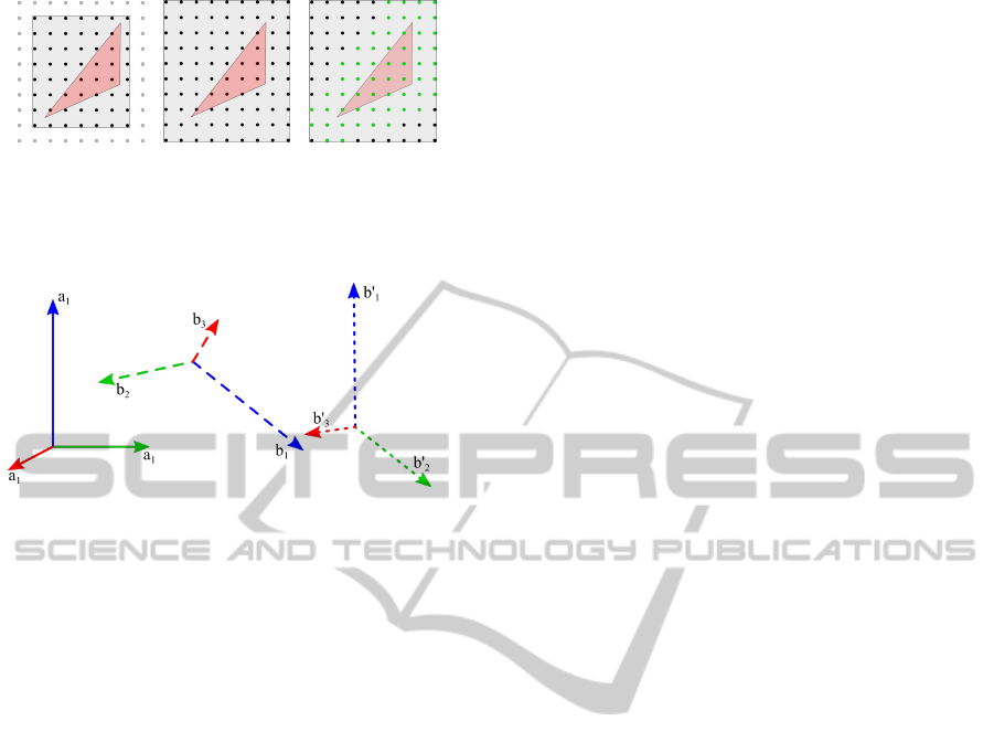
Figure 1: Left: the black nodes are the smallest subgrid

that completely contains the red face. Centre: the smallest

subgrid is extended to decrease discontinuities. Right: the

nodes highlighted in green are the imprint of the red face on

the lattice.

Figure 2: Left, solid: eigenbasis of mesh A. Centre, dashed:

eigenbasis of mesh B. Right, dotted: eigenbasis of mesh B

‘imprint’ of the mesh M on the lattice).

For each mesh imprint (from Figure 1; the collec-

tion of green nodes from every face in the mesh), we

perform PCA on the nodes’ coordinates and sort the

output eigenvectors in decreasing order of eigenvalue

magnitude. Note that a more sophisticated implemen-

tation of the algorithm would apply a weighted PCA,

with the weight of each node derived from its dis-

tances to the mesh triangles that pushed it in I

. How-

ever, we have found experimentally that this would

not have a signiﬁcant effect on the results and thus,

we opted for the much simpler unweighted PCA.

Between the two eigenbases (one for each mesh),

pairs of eigenvectors are formed based on them hav-

ing the largest, middle, or smallest eigenvalue magni-

tude (blue, green, and red correspondingly in Figure

2). Since PCA does not provide oriented principal

components, we have to ensure that the two eigen-

bases are consistently oriented. Where an inconsis-

tent orientation was detected, as we discuss in Sec-

tion 3.3, the sign of the eigenvector with the smallest

eigenvalue was ﬂipped in one of the meshes.

For the actual mesh alignment, we start with the

ﬁrst pair of principal components, a

, b

, (those with

the largest eigenvalues; blue). The rotation aligning

with b

(blue) is computed and applied to mesh B

to produce mesh B

. Lattice imprinting and PCA is

then performed on B

. The rotation around a

(or,

equivalently at this point, b

) aligning a

with b

(green) is then computed and applied to B

to produce

a mesh B

which is in alignment with A.

Note that it would have been possible to work out

both rotations (or even, a single rotation) from the ini-

tial PCA, however this is likely to be less accurate, as

the imprints of the meshes B and B

are different. In-

stead, by imprinting for a second time, the alignment

of the second eigenvector uses a dataset that is closer

to B

3.2 Iterative Algorithm

The basic algorithm can be repeated on mesh A and

the mesh B

(which has been aligned with A). The

procedure usually leads to a closer alignment, but the

decrease is not monotonic, and in some cases it could

even lead to poorer alignment.

We believe that the reason for the non-monotonic

decrease is the discrete nature of the grid relative to

the mesh itself, which means that even a tiny rotation,

which can change the position of any mesh vertex by

no more than an arbitrary small distance ε, may never-

theless change the position of a grid node marked for

processing by a distance equal to the edge of a grid

cell.

3.3 Eigenvector Orientation

In order for the method to work, the principal com-

ponents of meshes A and B must be consistently ori-

ented. However, PCA does not deﬁne a consistent

orientation. In order to align the two principal com-

ponents a

and b

consistently we evaluated a sum of

distances function on the two extreme mesh vertex

projections on the principal axis. For each of these

points, the distance to every data point was summed.

Then the principal axis was oriented in the direction

of the point with the largest associated sum.

Consistent orientation of principal components is

a particularly challenging problem. In our experi-

ments we noticed instances where the method was not

successful, causing large deviations (approximately π

radians) from the true alignment.

3.4 Input Types

The algorithm can, with minimal alteration, be used to

align a mesh with a point cloud, or even to align two

point clouds. Each point in the cloud is simply inter-

preted as a face with zero area. Here, the beneﬁt of

using the lattice instead of performing PCA directly

on the point cloud is the increased robustness of the

calculations due to the external reference. Which al-

lows, for example, the alignment of a point cloud and

a simpliﬁed version thereof.

GRAPP2015-InternationalConferenceonComputerGraphicsTheoryandApplications

176

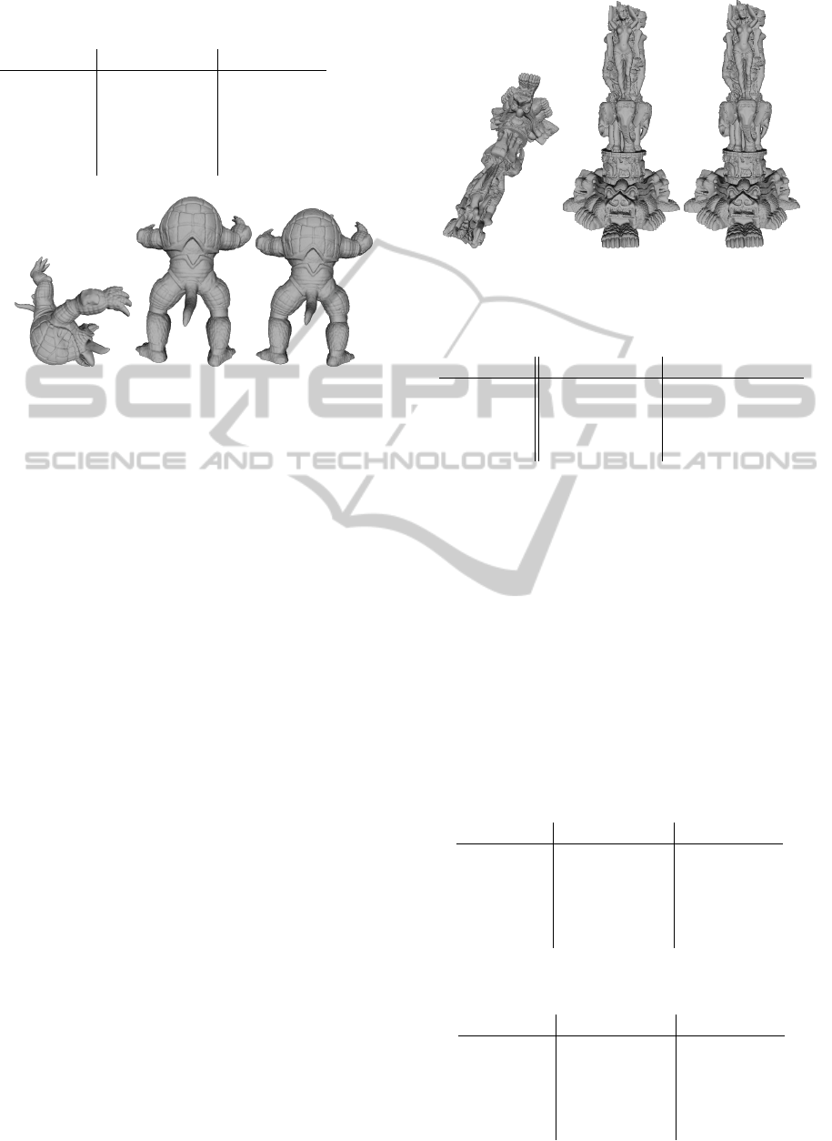
Table 1: Mean errors (in degrees) when recovering angles

from a set of known rotations.

Mesh Mesh Imprint Vertex PCA

Bunny 0.45407 0.00648

Armadillo 0.18480 0.01150

Fandisk 1.11274 0.00075

Blade 0.93554 0.00650

Statuette 5.62708 0.01968

Figure 3: Standard Armadillo results. Left: initial rotation,

middle: original, unrotated mesh, right: four iterations.

When working with a point cloud, the same pro-

cedure would be followed, but treating each point as a

face with no area, so the initial containing subgrid (P

above) would always be a single cube, which would

become a 3 × 3 × 3 subgrid after expansion.

4 RESULTS

In the ﬁrst experiment, each mesh had its principal

components computed by mesh imprinting and was

rotated by a known angle around the largest principle

component. The proposed algorithm was then used

to recover the rotation angle. This was then repeated

using vertex PCA and the results were compared. The

results are summarised in Table 1.

Since mesh alignment is an ill-posed problem, in a

second experiment we evaluated the visual relevance

of the reported errors by rotating the test meshes by

an unknown angle around an unknown axis. The

algorithm was used to bring them back into align-

ment. The results for the Armadillo and Statuette,

with the smallest and largest mean error respectively,

are shown in Figures 3 - 4.

4.1 Robustness against Mesh Processing

Operations

Smoothed versions of the models were obtained by

applying three iterations of Laplacian smoothing.

Simpliﬁed versions were obtained by using clustering

decimation with a cell size of 1% of the diagonal of

the bounding box. The decimation results are shown

Figure 4: Standard Statuette results. Left: initial rotation,

middle: original, unrotated mesh, right: four iterations.

Table 2: Number of faces in the original and decimated

meshes.

Mesh Original faces Decimated faces

Bunny 35,947 9,588

Armadillo 172,974 7,540

Blade 1,765,388 16,088

Statuette 10,000,000 18,330

in Table 2. Noisy meshes were obtained by randomly

displacing vertices by 1% of the bounding diagonal.

Finally, for remeshed models, surfaces were recon-

structed using the Poisson method (Kazhdan et al.,

2006) with 10 octree subdivisions.

The algorithms were then run against the each

mesh and the processed variants thereof. For each

method, the angular deviation between correspond-

ing principal components of the original and the pro-

cessed mesh were computed. The results are sum-

marised in Tables 3 - 6.

The proposed algorithm performed well on the

remeshed and simpliﬁed variants, but the noisy and

Table 3: Average deviation of principal components (in ra-

dians) when models were remeshed.

Remeshed Mesh Imprint Vertex PCA

Bunny 0.020450 0.044197

Fandisk 0.008237 0.008643

Armadillo 0.003517 0.014637

Blade 0.001020 0.018607

Statuette 0.063070 0.264650

Table 4: Average deviation of principal components (in ra-

dians) when models were simpliﬁed.

Simpliﬁed Mesh Imprint Vertex PCA

Bunny 0.008457 0.031510

Fandisk 0.024567 0.116733

Armadillo 0.002427 0.007957

Blade 0.005060 0.008093

Statuette 0.017803 0.300917

MeshAlignmentusingGridbasedPCA

177

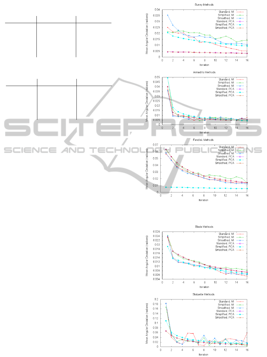
Table 5: Average deviation of principal components (in ra-

dians) when mesh vertices had noise added.

Noisy Mesh Imprint Vertex PCA

Bunny 0.001363 0.000333

Fandisk 0.000047 0.000240

Armadillo 0.000563 0.000757

Blade 0.000753 0.000357

Statuette 0.004997 0.000267

Table 6: Average deviation of principal components (in ra-

dians) when meshes were simpliﬁed.

Smoothed Mesh Imprint Vertex PCA

Bunny 0.012873 0.000170

Fandisk 0.006650 0.000080

Armadillo 0.003757 0.000800

Blade 0.000270 0.000107

Statuette 0.001483 0.000000

smoothed variants were better served by vertex PCA.

This is in line with our expectations as remeshing and

simpliﬁcation are likely to have a larger impact on

vertex distribution than uniformly applied noise and

smoothing.

4.2 Iterative Algorithm

The performance of the iterative algorithm is shown in

Figures 5 and 6. We notice that generally, the itera-

tive algorithm has improved accuracy in each succes-

sive iteration and that most of the improvement mate-

rialises in the ﬁrst three or four iterations.

Of particular note are the simpliﬁed Fandisk re-

sults in Figure 5. Whilst Vertex PCA appears to in-

stantly converge to a highly accurate result, in real-

ity this was a very poor alignment - the simpliﬁed

Fandisk had many large, thin triangles. This signif-

icantly altered the distribution of vertices in the mesh

and makes the comparison of the two sets of principal

components invalid. The Mesh Imprint results on the

simpliﬁed mesh are a true representation of the align-

ment, as are the Vertex PCA results for the standard

and smoothed Fandisk.

4.3 CAD Meshes

The proposed method is particularly well suited for

CAD meshes that have undergone mesh processing

operations. The Room 215 model shown in Figure 7

is a hand-made replica of an ofﬁce created using CAD

software, it has 171,711 faces and signiﬁcant variance

in vertex density. For instance, large areas of walls

are represented by huge triangles, but tiny triangles

are used to pick out the detail and high-curvature of

the radiator grills and chairs. The simpliﬁed form has

Figure 5: Mean angular deviation plotted against number of

iterations for the Bunny, Armadillo and Fandisk.

Figure 6: Mean angular deviation plotted against number of

iterations for the Blade and Statuette.

GRAPP2015-InternationalConferenceonComputerGraphicsTheoryandApplications

178

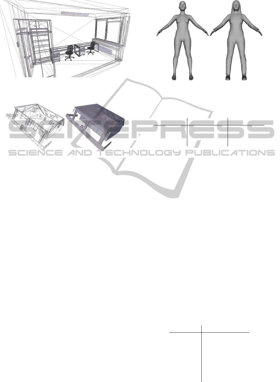
Figure 7: Wireframe view of the Room 215 model. Areas

of high curvature have more triangles and appear as solid

colours.

Figure 8: Wireframe view of the original House model and

its remeshed form.

16,080 faces.

When the principal components of each were

computed and compared, Mesh Imprinting proved

very effective, with a maximum deviation of 0.0086

radians across all principal components, compared to

a minimum deviation of 0.11 radians for vertex PCA.

The same test was run against a simple house

model and a remeshed form thereof shown in Fig-

ure 8. The original mesh had 1,396 faces, the

remeshed model had 98,818. The maximum devi-

ation between the standard house and the remeshed

form thereof was 0.075 radians. Vertex PCA had a

minimum deviation of 0.12.

The model/dressed models in Figure 9 are a pair

of models that both depict a human ﬁgure. This ﬁg-

ure is nude in the regular model, but has long hair

and is wearing bulky/baggy clothes in the second.

Both were analysed and had their principal compo-

nents compared. The computation was reasonably

stable for both models, showing only small devia-

tions between the two meshes, but with up to ﬁve

times smaller deviations being produced by the mesh

imprint. The maximum deviation between principal

components computed by imprinting was 0.0022 radi-

ans, and the minimum computed by vertex PCA was

0.012.

This is not too surprising, as the two ﬁgures have

the same pose and the changes from the regular model

Figure 9: Model/dressed model.

Table 7: Mean angular deviations (in radians) between the

simpliﬁed and standard Room215, standard and remeshed

House, and standard and dressed Model.

Mesh Mesh Imprint Vertex PCA

Room 215 0.00647 0.11853

House 0.06064 0.20983

Model 0.00331 0.01230

to the dressed model are relatively rotationally sym-

metric between the two minor principal components.

The largest principal component is along the height

of the model, and the proportions do not change suf-

ﬁciently to make much difference to this.

4.4 Effect of Resolution

We experimented on grids at 10%, 50%, 100%, and

150% of their original size. The initial size (100%)

of each grid is shown in Table 8. In addition to the

meshes used earlier, the Sphere and Vase models (Fig-

ure 10) were also used.

Predictably, lower-resolution analyses usually

produced alignments that were not so accurate as

higher-resolution analyses. However for the Bunny

and Armadillo models the 150% resolution align-

ments were actually slightly less accurate than the

100% resolution analyses.

The Vase, Sphere and Statuette all highlighted a

limitation of the eigenvector orientation method; they

produced inaccurate results as one principal compo-

Table 8: Initial grid sizes.

Mesh Volume

Bunny 78 × 77 × 60

Armadillo 127 × 151 × 115

Fandisk 121 × 131 × 67

Blade 352 × 598 × 274

Statuette 235 × 396 × 203

Sphere 105 × 108 × 105

Vase 55 × 101 × 55

MeshAlignmentusingGridbasedPCA

179

Figure 10: Sphere and Vase.

nent was incorrectly aligned. This occurs when the

input meshes have high levels of rotational symmetry.

When run at an appropriate resolution the algorithm

correctly orients the principal components, leading to

a successful alignment. However there appears to be

no universally optimal resolution for the lattice in this

regard.

5 DISCUSSION

The implementation of each algorithm was not opti-

mised due to the wide variety of different techniques

and circumstances under which each is possible and

appropriate.

Our implementations took the simple approach of

reading the full ﬁle from the hard drive, processing the

data entirely in memory, and writing the output back

to the hard drive in a single execution thread. While

processing large meshes can require large amounts of

memory due to the sheer number of points that must

be processed, our method (by virtue of performing

PCA on fewer points) will naturally have a smaller

memory footprint. Memory could also be saved by

running the proposed algorithm in a layered fashion,

as proposed in (Kaye and Ivrissimtzis, 2011).

Since the proposed method aligned the meshes on

a relatively coarse regular grids, the loss of accuracy

compared to direct vertex PCA was noticeable, but

was inside a range that would be considered tolera-

ble in most applications, that is, around one degree if

there were no problems caused by the rotational sym-

metry of the meshes, or by wrongly oriented eigen-

vectors. Note that these problems are common to both

the proposed method and standard PCA on mesh ver-

tices.

Mesh Imprinting shows its strengths when orig-

inal inputs are poorly meshed, for instance, if they

have many long, thin triangles, or an uneven distribu-

tion thereof. While long thin triangles are very rare

in meshes that are acquired through physical optical

devices such as laser scanners, they often dominate

meshes produced by CAD software. In such cases,

simpliﬁcation and remeshing signiﬁcantly affect the

distribution of the vertices, causing Vertex PCA to

produce highly inaccurate alignments.

In the future we plan a systematic analysis of the

error of the standard PCA caused by vertex quantisa-

tion. Indeed, the small alignment error produced by

our method is essentially a vertex coordinate quan-

tisation error, which anyway may be present in the

vertex coordinates, if for example the mesh had un-

dergone lossy compression. By showing, as we con-

jecture, that the alignment error of our method and the

vertex PCA error caused by vertex coordinate quanti-

sation are comparable, we will further justify our ap-

proach.

ACKNOWLEDGEMENTS

The Room215 model is from the Max Planck Insti-

tute. The House mesh was created by user “pabong”

and downloaded from www.tf3dm.com. The model

and dressed model were created using the MakeHu-

man software from www.makehuman.org. The Vase,

Sphere, Statuette, and Blade models were taken from

the AIM@SHAPE repository.

REFERENCES

Ankerst, M., Kastenm

uller, G., Kriegel, H.-P., and Seidl,

T. (1999). 3D shape histograms for similarity search

and classiﬁcation in spatial databases. In Advances in

Spatial Databases, pages 207–226. Springer.

Besl, P. J. and McKay, N. D. (1992). A method for registra-

tion of 3-d shapes. IEEE Trans. Pattern Anal. Mach.

Intell., 14(2):239–256.

Cantoni, V., Gaggia, A., and Lombardi, L. (2013). Extended

gaussian image. In Encyclopedia of Systems Biology,

pages 724–725. Springer.

Cignoni, P., Callieri, M., Corsini, M., Dellepiane, M.,

Ganovelli, F., and Ranzuglia, G. (2008). Meshlab:

an open-source mesh processing tool. In Sixth Euro-

graphics Italian Chapter Conference, pages 129–136.

Elad, M., Tal, A., and Ar, S. (2002). Content based retrieval

of vrml objects: an iterative and interactive approach.

In Proceedings of the sixth Eurographics workshop on

Multimedia 2001, pages 107–118. Springer-Verlag.

Gelfand, N. and Rusinkiewicz, S. (2003). Geometrically

stable sampling for the icp algorithm. In Proc. Inter-

national Conference on 3D Digital Imaging and Mod-

eling, pages 260–267.

Hyv

arinen, A., Karhunen, J., and Oja, E. (2001). Indepen-

dent Component Analysis. Wiley-Interscience.

Kaye, D. P. and Ivrissimtzis, I. (2011). Memory Efﬁ-

cient Surface Reconstruction Based on Self Organ-

ising Maps. In Theory and Practice of Computer

Graphics, pages 25–32.

Kazhdan, M., Bolitho, M., and Hoppe, H. (2006). Poisson

surface reconstruction. In SGP ’06, pages 61–70.

GRAPP2015-InternationalConferenceonComputerGraphicsTheoryandApplications

180

Kazhdan, M., Funkhouser, T., and Rusinkiewicz, S. (2003).

Rotation invariant spherical harmonic representation

of 3D shape descriptors. In SGP ’03.

Maier-Hein, L., Santos, T. R. D., Franz, A. M., and Meinzer,

H.-P. (2010). Iterative closest point algorithm in the

presence of anisotropic noise. In Bildverarbeitung f

die Medizin, pages 231–235.

Papadakis, P., Pratikakis, I., Perantonis, S., and Theoharis,

T. (2007). Efﬁcient 3d shape matching and retrieval

using a concrete radialized spherical projection repre-

sentation. Pattern Recogn., 40(9):2437–2452.

Postelnicu, G., Zllei, L., and Fischl, B. (2009). Combined

volumetric and surface registration. IEEE Trans Med

Imaging, 28(4):508–22.

Roy, M., Foufou, S., and Truchetet, F. (2004). Mesh com-

parison using attribute deviation metric. Journal of

Image and Graphics, 4:1–14.

Rusu, R. B. and Cousins, S. (2011). 3D is here: Point Cloud

Library (PCL). In IEEE International Conference on

Robotics and Automation (ICRA).

Sahambi, H. S. and Khorasani, K. (2003). A neural-

network appearance-based 3-d object recognition us-

ing independent component analysis. IEEE Trans.

Neur. Netw., 14(1):138–149.

Sﬁkas, K., Theoharis, T., and Pratikakis, I. (2014). Pose

normalization of 3d models via reﬂective symmetry

on panoramic views. The Visual Computer, pages 1–

14.

Vranic, D., Saupe, D., and Richter, J. (2001). Tools for 3d-

object retrieval: Karhunen-loeve transform and spher-

ical harmonics. In Workshop on Multimedia Signal

Processing.

MeshAlignmentusingGridbasedPCA

181