Optimization-based Automatic Segmentation
of Organic Objects of Similar Types
Enrico Gutzeit, Martin Radolko, Arjan Kuijper and Uwe von Lukas
Fraunhofer Institute for Computer Research IGD, Joachim-Jungius-Str. 11, 18059 Rostock, Germany
Keywords:
Image Segmentation, Application, Graph Cut, Belief Propagation.
Abstract:
For the segmentation of multiple objects on unknown background in images, some approaches for specific
objects exist. However, no approach is general enough to segment an arbitrary group of organic objects of
similar type, like wood logs, apples, or tomatoes. Each approach contains restrictions in the object shape,
texture, color or in the image background. Many methods are based on probabilistic inference on Markov
Random Fields – summarized in this work as optimization based segmentation. In this paper, we address the
automatic segmentation of organic objects of similar types by using optimization based methods. Based on
the result of object detection, a fore- and background model is created enabling an automatic segmentation of
images. Our novel and more general approach for organic objects is a first and important step in a measuring
or inspection system. We evaluate and compare our approaches on images with different organic objects on
very different backgrounds, which vary in color and texture. We show that the results are very accurate.
1 INTRODUCTION
The segmentation of multiple objects on unknown
background in images is a hard and unresolved prob-
lem in computer vision. There exist some approaches
for specific objects like wood logs, apples, or toma-
toes. However, no approach is general enough to seg-
ment an arbitrary group of organic objects of similar
type. Each approach contains restrictions in the object
shape, texture, color or in the image background.
To overcome this limitation, we propose to re-
lax the restrictions with a general and novel approach
based on an object detection and optimization based
segmentation. “Optimization based methods” is the
terminology we use to summarize the methods based
on probabilistic inference on Markov Random Fields.
These methods optimize a segmentation by using
probability maps or presegmented images.
In this paper, we address a specific class of ob-
jects, namely a group of organic objects of similar
type, such as fruits, wood log surfaces, or fishes. We
coin such a group of objects in short “organo-group”
(see section 3 for details). In Figure 1 four different
organo-groups are shown.
The segmentation of an organo-group is an impor-
tant step in inspection, measurement, or recognition
for industrial or research applications. For example,
the volume of a wood stack, the sizes of fishes, or
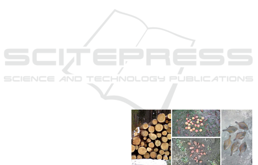
Figure 1: The picture shows four different groups of organic
objects of similar types (organo-groups), namely wood cut
surfaces, apples, potatoes and flatfishes.
the number of apples can be estimated after success-
ful segmentation. The segmentation is most often the
first step in a full measuring or inspection system.
In this paper, we introduce our approach, which
is split into the parts organic object detection, veri-
fication, optimization based segmentation and object
separation.
In the following sections, we analyze related work
and discuss the remaining problems in the subsequent
section. We then introduce our approach and its steps.
Next, we present and compare the results we get by
adapting graph-cut and belief propagation on the seg-
mentation of the four different types of organo-groups
shown in Figure 1, viz. wood log surfaces, fishes,
potatoes, and apples. Finally, we give a conclusion.
591
Gutzeit E., Radolko M., Kuijper A. and von Lukas U..
Optimization-based Automatic Segmentation of Organic Objects of Similar Types.
DOI: 10.5220/0005314905910598
In Proceedings of the 10th International Conference on Computer Vision Theory and Applications (VISAPP-2015), pages 591-598
ISBN: 978-989-758-089-5
Copyright
c
2015 SCITEPRESS (Science and Technology Publications, Lda.)

2 RELATED WORK
There are miscellaneous classifications of the basic
segmentation methods, depending on the point of
view of the user. From our point of view, there are
four main classes: the pixel-based, contour-based,
region-based and optimization based methods. Pixel-
based methods segment pixel per pixel. Well-known
examples are thresholding techniques (Otsu, 1979;
Sezgin and Sankur, 2004). Contour-based methods
locate, analyze and / or merge contours. An exam-
ple are snakes (Kass et al., 1988; Chan and Vese,
2001). Region-based methods group similar pixels to
regions. Examples are the well-known watershed and
the SLIC approach (Achanta et al., 2012). Another,
but sill similar type is object detection (Zhang et al.,
2013), which mostly use an trained object model to
locate objects in the image.
In this paper, we address optimization based seg-
mentation, which contains the methods based on a
statistical model, especially a Markov Random Field
(MRF) (Li, 1995). Well-known methods of the op-
timization based segmentation class are graph-cut
(Boykov and Kolmogorov, 2004), normalized cut (Shi
and Malik, 2000), belief propagation (Felzenszwalb
and Huttenlocher, 2006) and Fields of Expert (Roth
and Black, 2005). The disadvantage of these meth-
ods is that they normally do not automatically seg-
ment an image and need additional input, like proba-
bility maps or user defined regions. An example for
a semi-automatic graph-cut segmentation is the grab-
cut approach in (Rother et al., 2004). Here, an object
is segmented after a user has drawn a rectangle around
the object.
In contrary to the basic methods, the application-
driven methods are hardly classified by algorithmic
similarity. The best way for classification is the ap-
plication itself. A generic segmentation of an organo-
group does not exist and is thus not state of the art,
but specific groups are addressed in image processing
literature.
Some approaches exist to segment wood cut sur-
faces. An adaptive local threshold over the image is
used in (Medina Rodriguez et al., 1992). In (Dahl
et al., 2006) a watershed and an automatic scale space
selection is adapted to solve the problem. In (Gutzeit
et al., 2010) the center image is first segmented and
the results are then used to create a fore- and back-
ground model. With these models the whole image is
binary segmented (wood / non wood) by the graph-
cut method. This approach needs to have wood logs
in the center of the image. It was extended in (Gutzeit
and Voskamp, 2012) by relaxing these restrictions us-
ing an object detection to estimate the center region
of the stack of wood. Each individual wood log is
segmented in contrast to the complete wood area. In
(Herbon et al., 2014) an iterative detection and seg-
mentation approach for wood-logs by using different
classifiers is introduced. The approach lead to very
good results, but need well trained classifiers.
The segmentation and detection of fruit objects is
addressed in (Zhao et al., 2005; Wijethunga et al.,
2008; Rui et al., 2010; Akin et al., 2012; Aloisio
et al., 2012) – each addressing a specific fruit type. A
texture-based object detection by using the gray level
co-occurrence matrix is adapted in (Zhao et al., 2005;
Rui et al., 2010) to detect and segment apples. A spe-
cial and heuristic color range of the RGB color space
is used in (Akin et al., 2012) to detect apples. Another
heuristic color range is applied in (Wijethunga et al.,
2008) to segment kiwis. Especially, cluster of the a
and b channels of the Lab-color space are first trained
for kiwis. Then, the distance to the trained cluster is
used to segment the fruits. In (Aloisio et al., 2012)
citrus fruits are pixel-wise segmented with a Bayes
classifier.
The segmentation of fishes is rarely addressed in
research. Existing approaches are mostly designed
for underwater imaging (Lee et al., 2010; Zhu et al.,
2012). In both approaches, the frame to frame coher-
ence is used in videos to segment the moving fishes.
An approach based on single images and individual
fishes is introduced in (White et al., 2006) for the
segmentation of caught fishes lying on a convey belt.
First, the major color range in the RGB color space of
the conveyer belt is calculated in a calibration step. In
the segmentation step, a pixel outside the color space
is segmented as fish pixel, if 40% of the pixels in a
10 ×10 neighborhood are also outside the threshold.
In summary, many methods to segment organo-
groups exist, but all methods are very specialized.
They only work under specific conditions and are
mostly designed for a specific organo-group.
3 ORGANO-GROUPS
In our scenario, a picture of one organo-group is taken
by e.g. a mobile phone. We cannot address all kinds of
organo-groups, but select a subset to validate our ap-
proach. This means, we especially address potatoes,
apples, flatfishes and wood cut surfaces. Most objects
of the groups are located on an arbitrary background
(e.g. grass, stone floor, sand). In the case of wood
cut surfaces, a picture of the front side of a stack of
wood is taken. The objects of the organo-groups we
examine:
• overlap each other not more then 20%
VISAPP2015-InternationalConferenceonComputerVisionTheoryandApplications
592

• are quasi round, which means, that the overlap of
the best fitting circle with the same area is greater
than 60%
• are of the same kind (species) and mostly similar
in texture and color
Figure 2: Pictured is a subset of the organic objects (wood
cut surfaces, flatfishes, apples and potatoes) of our scenario.
The objects are different in shape, color and texture. Also
the background is different and unknown.
In one image the objects of one organo-group are
similar, but yet there is a certain variance between
the objects in color, shape and texture. Furthermore,
the characteristics of one organo-group to another
organo-Group are completely different, e.g. wood
logs in compare to flatfishes. And last but not least,
the background is unknown and varies in color and
texture. Some objects of each group can be seen in
Figure 2.
4 OUR APPROACH
Our more generalize approach extends the specific
approach for wood log segmentation in (Gutzeit and
Voskamp, 2012). Similar as in the wood log segmen-
tation case, the objects of a specific organo-group in
one image are mostly similar in color and texture. For
that reason, we think that an optimization-based seg-
mentation with an appropriate color model is a good
way to solve the problem. In our approach we cre-
ate a color model of the objects (foreground) and non
objects (background) by using an simple object detec-
tion and verification method. Based on this model, a
probability map of fore- and background is calculated
with a special sampling approach. The image is then
binary segmented by an optimization-based method
and the objects are finally separated. The four steps
of our approach are illustrated in Figure 3.
Figure 3: Our principal methodology and the steps of our
organo-group segmentation.
In the first step, the organic objects are detected
by a trained detector. We have decided to use haar-
cascades (Viola and Jones, 2001) as a detector, be-
cause they allow the training of a moderate detector
with only a few samples. The detection in our ap-
proach does not have to be very robust, but should
detect approximately 50 % of the objects. Further-
more, the detected objects are verified by removing
outliers and solving overlaps. The result is a set of
circles C, which is used in the second step to cre-
ate two models. One model contains estimated pix-
els of the foreground and the other one the pixels of
the background. Based on these models and a density
estimation, two probability maps (I
f g
, I
bg
) are cre-
ated. In the third step, the image is binary segmented
with different optimization-based approaches involv-
ing I
f g
and I
bg
. We especially apply graph-cut (GC)
and belief propagation (BP). Finally, the objects are
separated in the fourth step.
In the case of wood logs, the objects (wood cut
surfaces) are grouped in image space, have a high
yellow value and are brighter as the space between
the wood logs. In the general scenario the assump-
tion does not hold, because the organic objects can be
scattered and the color of the objects is unknown. We
thus generalize and improve the following parts (cf.
Figure 3):
• another object verification method to optimize the
true positive rate,
• an easier and more general method to estimate
pixels of the fore- and background usable to create
color models for segmentation, and
• an improved object separation method.
Additionally, we apply belief propagation to show the
general aspect and to find the best optimization based
method for our purpose. For this, we use probability
maps of the fore- and background as interface to the
optimization based segmentation method.
4.1 Object Detection and Verification
In the original wood log segmentation approach, the
wood cut surfaces are detected by well trained haar-
cascades. After that, to optimize the true positive
rate, the detected objects are verified by eliminating
outliers and overlapping objects. In our scenario the
objects are scattered and not grouped as wood logs.
Hence, an outlier elimination in image space is not
reasonable. Therefore, we also detect the objects,
but verify them by using the color similarity. We
decided us to apply haar-cascades (Viola and Jones,
2001) as detector, because a training set of 100 pos-
itive and 300 negative samples are enough to get a
moderate detector and the creation of some samples
is usually not a hard task. The detection with the
Optimization-basedAutomaticSegmentationofOrganicObjectsofSimilarTypes
593

trained haar-cascades leads to a set of rectangles. To
improve the detection result, we first convert the rect-
angles with width w and height h into a set of circles
C. The radius r of one circle is calculated by
w+h
2
and the center of the circle corresponds to the center
of the rectangle. Next, we apply a special verifica-
tion of the circles in terms of color similarity. For
every circle the mean color of a pixel in RGB color
space px
m
= (r
m
,g
m
,b
m
)
T
is calculated. The circles
are therefore scaled down first by r = r ·0.75 to get
only pixels of the object. Then, the mean and vari-
ance over all n circle mean colors is calculated:
px =
1
n
n
∑
i=1
px
m
i
; σ
px
=
1
n
n
∑
i=1
k
px − px
m
i
k
2
;n = |C|
(1)
The circles with the greatest Euclidean distance
to the mean is removed. The process is repeated un-
til the variance σ
px
is under a certain threshold T .
It experimentally turned out, that T = 20 is a good
threshold for images with r,g,b ∈ [0, 255]. We note
that objects in our scenario only slightly overlap each
other. The overlap from one to another object in C is
normally not greater than 20%. Consequently, we re-
move all smaller objects with an greater overlap. The
two described simple outlier removing methods lead
to fewer false-positive detections (see Figure 4).
Figure 4: The results of the detection (upper row) and ver-
ification step (lower row) of wood cut surfaces, flatfishes,
potatoes and apples.
4.2 Fore- and Background Estimation
The aim of this step is to estimate a foreground
(FG
smp
) and a background pixel set (BG
smp
). With
the pixel sets, the image can be binary segmented with
a kd-tree accelerated density estimation (KD-NN) fol-
lowed by an optimization based segmentation. This
method by using graph-cut applied on wood logs is
called KD-NN-A in (Gutzeit and Voskamp, 2012). In
the KD-NN-A approach, a trimap I
tri
is used to mark
a pixel as unknown, foreground or background. The
foreground pixels are calculated with a heuristic color
segmentation followed by a graph-cut segmentation
on a certain region around the mean of the verified
objects. In contrast to the foreground pixels, the back-
ground pixels are calculated through a distance trans-
form.
In this approach, we estimate the pixels in an
easier way without color heuristics and a graph-cut
presegmentation. Furthermore, we calculate first a
trimap and than a foreground (I
f g
) and background
probability map (I
bg
) by using the KD-NN. A proba-
bility map contains probabilities p ∈[0,1]. Each pixel
of the image I
in
corresponds to one foreground (p
f g
∈
I
f g
) and to one background probability (p
bg
∈ I
bg
).
Both maps are an independent interface to the next
step, the optimization based segmentation. We call
this approach KD-NN-G (KD-NN-generalized).
In our approach, we create the trimap I
tri
by ran-
dom sampling with the set C. One label l in I
tri
cor-
responds to one in I
in
and can have the value u (un-
known), f g (foreground) or bg (background). Each
circle c ∈ C is represented by a triple c = (x
c
,y
c
,r),
whereby (x
c
,y
c
)
T
is the center position and r the ra-
dius. The labels in I
tri
are set for each pixel in I
in
at
position (x,y)
T
by using a threshold a ∈ [0,1]:
f (~p,C,a) =
f g, ∃(~p
c
,r) ∈C : k~p −~p
c
k
2
< a ·r
u, ∃(~p
c
,r) ∈C : k~p −~p
c
k
2
∈ [a ·r,r]
bg, otherwise
(2)
It experimentally turned out that a = 0.7 is a good
threshold. All pixels in I
in
marked with l = f g are put
into the pixel set FG and for l = bg into BG. The pixel
sets are normally not equal in size and can hold falsely
classified pixels. The usually unwanted case is that
a non-detected object is marked as background. To
weaken the influence of falsely classified pixels, we
apply a random sampling over BG and FG. The re-
sults are two subsets of equal size FG
smp
and BG
smp
.
The size of the subsets is relative to the image width
(w) and height (h) in the following way:
w ·h ·b = |FG
smp
| = |BG
smp
|; b ∈[0,1] (3)
FG
smp
⊆ FG; BG
smp
⊆ BG (4)
A good scaling factor is b = 0.05. All pixels,
which are not in FG
smp
or BG
smp
are set in I
tri
to
u (unknown) and all pixels in FG
smp
and BG
smp
are
stored in two separate kd-trees. Finally, the probabil-
ity maps I
f g
and I
bg
are created by a density estima-
tion with a sphere environment on the kd-trees.
VISAPP2015-InternationalConferenceonComputerVisionTheoryandApplications
594

4.3 Graph-Cut and Belief Propagation
Using the probability maps created in the last step, the
aim of this step is to binary segment the input image
I
in
and adapting an optimization based segmentation.
We therefore adapt two different methods, graph-cut
and belief propagation.
A graph-cut (GC) is a cut of a graph G = (V,E)
with the nodes V and weighted edges E. The nodes V
consists of non-terminal (pixel nodes) and two termi-
nal nodes (source s and sink t). A pixel node cor-
responds to an image pixel and is connected to its
four neighbors. A terminal node is connected to all
pixel nodes, whereby s represents foreground and t
background. We directly set the edge weights from a
terminal node to a non-terminal node with the corre-
sponding probabilities in I
f g
and I
bg
. The weights w
between the non-terminal nodes are set with
w = 1 −e
−α·
k
px
i
−px
j
k
, (5)
where px = (r,g,b)
T
denotes a pixel in the RGB color
space, α is a free scaling factor and i, j are adjacent
non-terminal nodes. A suitable value for α is 0.0005.
After the graph weighting, the min-cut/max-flow of
(Boykov and Kolmogorov, 2004) is applied.
For the belief propagation (BP), we adapt the
loopy max-product BP algorithm of (Felzenszwalb
and Huttenlocher, 2006). The algorithms works by
parsing messages around a four connected image
graph. A message from nodes i to the connected node
j is denoted by m
k
i→j
, whereby k denotes the iteration.
Our message has two dimensions due to the two pos-
sible labels L = {0,1}. 1 labels a object pixel and 0 a
non-object pixel. One message is computed in a sim-
ilar way as in (Felzenszwalb and Huttenlocher, 2006)
at each iteration:
h(l
j
,l
i
) = c ·ψ(l
j
,l
i
) + c ·φ(l
i
) +
∑
s∈N( j)\i
m
k−1
s→j
(l
j
)
m
k
j→i
(l
i
) = min
l
i
(h(l
j
,l
i
))
(6)
We extent Eq. (6) by the scaling factor c = 0,9 to
force convergence and to stronger weight the starting
state. l
i
,l
j
∈ L are the labels of node i and j. In our
case, the discontinuity cost ψ of two adjacent nodes
and the matching cost φ are computed by:
ψ(l
i
,l
j
) =
(
0, l
i
= l
j
1, l
i
6= l
j
; φ(l
i
) =
(
1 − p
f g
i
, l
i
= 1
1 − p
bg
i
, l
i
= 0
(7)
whereby p
i
denotes the corresponding probability in
I
f g
or I
bg
of the node i. The final belief is calculated
as in (Felzenszwalb and Huttenlocher, 2006).
Figure 5: left: the input image I
in
, middle: I
b
, the result
of the GC (left) and BP (right) segmentation, right: I
og
, the
result of the GMC-G separation on the GC result.
The result of both optimization based methods are
a binary image I
b
with object pixels (l = 1) and non-
object pixels (l = 0), which is illustrated in Figure 5.
4.4 Object Separation with GMC-G
In this last step, the objects are separated by using
the verified circles C in the binary image I
b
(l ∈
{0,1}). We generalized the LSGMC (Log Separa-
tion by Growing Moving Circles) approach described
in (Gutzeit and Voskamp, 2012) and call the extended
one GMC-G (GMC-generalized). The LSGMC is op-
timized for the separation of wood cut surfaces in a
binary image I. The approach fits circles C together
with extracted local maxima into an binary image
I
b
. The local maxima are calculated by a distance-
transform and converted into circles. All circles to-
gether simultaneously grow, move and melt until a
certain energy is reached, which means the ratio be-
tween a circle and the underlying segmented pixels
(l = 1). The circle fitting part is called GMC (Grow-
ing Moving Circles).
The major problem of the LSGMC is that non-
round objects will be split into unwanted parts (under-
segmentation). To solve this problem, we additionally
add first order statistics of the circle set C and a wa-
tershed segmentation. Especially, we use the mean r
and variance σ
r
of the circle radii in C.
First, all pixels inside a circle c ∈C in I
b
are set to
0 and a distance-transform is processed on the result-
ing binary image. Then, the distance image is thresh-
old segmented by T = max (r −3σ
r
,r/2). The out-
come of the segmentation are those segments S which
are probably non-detected objects. For all S, the mass
center mc = (x
m
,y
m
)
T
and radii r
s
=
√
A ÷π are cal-
culated. The symbol A represents the area as well as
the amount of pixels in S. Each S is united as circle
c
s
= (x
m
,y
m
,r
s
) with C. The result is an extended set
C
e
which is subsequently fit into the image I
b
by us-
ing the GMC. The fitted circles C
f
are further used
to determine seed points for a watershed segmenta-
tion. Especially, we determine a marker image I
m
with |C
f
|+ 2 labels. Each label in I
m
inside a circle
(x,y,0.8 ·r) ∈C
f
is set to the circle index. All other
labels are set to unknown (−1). Furthermore, the la-
Optimization-basedAutomaticSegmentationofOrganicObjectsofSimilarTypes
595

bels in I
m
, which are background in I
b
and more than
3·σ
r
pixels away from the nearest object pixel, are set
to 0. Finally, the image I
in
is watershed segmented by
using I
m
. The results on some examples in our data
set can be seen on the right of Figure 5.
5 Results
The detection, verification and segmentation results
are evaluated against the ground truth (GT). We all-
together use 71 wood log, 25 potatoes, 25 apples and
25 flatfish images. In all images the background and
objects are different in color, texture, and shape. We
separately evaluate the object verification, segmen-
tation, and separation step. For the evaluation we
mainly use the measures precision, recall, and f-score.
Additionally, to evaluate the separation (multi-object-
segmentation) the HD-M (Huang-Dom-measure in
(Huang and Dom, 1995)) is used. In all measures, the
best value is 1 and the worst one is 0. Some results of
our approach in comparison to grab-cut are illustrated
in Figure 6.
5.1 Object Detection and Verification
The objects are detected with haar-cascades and are
subsequently verified. Table 1 shows the average pre-
cision, recall, and f-score we get for the detected (up-
per table) and verified objects (lower table). The stan-
dard deviation is presented in brackets.
Table 1: Detected (upper table) and verified (lower table)
organic objects.
object precision recall f-score
wood 0.81 (0.1) 0.69 (0.11) 0.745 (0.1)
apple 0.97 (0.04) 0.95 (0.06) 0.96 (0.05)
potato 0.70 (0.18) 0.59 (0.27) 0.60 (0.21)
flatfish 0.94 (0.11) 0.66 (0.21) 0.76 (0.17)
wood 0.87 (0.07) 0.68 (0.11) 0.76 (0.09)
apple 0.97 (0.04) 0.94 (0.06) 0.95 (0.04)
potato 0.88 (0.2) 0.57 (0.27) 0.65 (0.24)
flatfish 0.96 (0.09) 0.65 (0.21) 0.76 (0.17)
The values related to the detected objects are
mostly between 0,6 and 0,75. The best results are
achieved with apples. The detection of apples is
nearly perfect, because apples have a round shape and
mostly a homogenous color. After the object verifica-
tion step the f-score and the precision is better in all
cases excluding the apples. In the apple case, only
the f-score is a little bit poorer as before. To create
a good foreground model for the segmentation, valid
object samples are needed. For that reason, the preci-
sion of the detection is more important than the recall.
This means regarding to the results the verification of
the objects is an useful and appropriate step.
5.2 Binary Object Segmentation
The result of the optimization based segmentation
(BP, GC) is a binary image. To evaluate the binary
segmentation we use again precision, recall, and f-
score. Different to the object verification evaluation,
the pixels (object or non object) and not the object
itself are taken into account.
In our approach, the final binary segmentation can
be done with graph-cut (GC) or belief propagation
(BP) based on our KD-NN-G. The results of both
methods are illustrated in Table 2.
Table 2: Evaluation of the binary segmentation (classifica-
tion as object or non object pixel). The best values are in
bold print.
object precision recall f-score
KD-NN-A with GC
wood 0.88 (0.08) 0.95 (0.03) 0.91 (0.04)
apple 0.97 (0.03) 0.70 (0.19) 0.80 (0.12)
potato 0.41 (0.47) 0.24 (0.29) 0.29 (0.35)
flatfish 0.19 (0.37) 0.08 (0.2) 0.09 (0.16)
KD-NN-G with BP
wood 0.77 (0.09) 0.94 (0.04) 0.85 (0.07)
apple 0.88 (0.19) 0.71 (0.19) 0.74 (0.13)
potato 0.91 (0.07) 0.76 (0.09) 0.82 (0.05)
flatfish 0.96 (0.07) 0.69 (0.1) 0.8 (0.08)
KD-NN-G with GC
wood 0.92 (0.04) 0.92 (0.05) 0.92 (0.03)
apple 0.98 (0.01) 0.89 (0.08) 0.94 (0.05)
potato 0.93 (0.05) 0.87 (0.06) 0.9 (0.04)
flatfish 0.97 (0.08) 0.82 (0.1) 0.88 (0.08)
The results with the adapted belief propagation
method are in general not as good as the results us-
ing graph-cut, but still suitable with an average f-
score of 0.8. This shows, that different optimization
based methods can be applied to solve the problem,
whereby graph-cut leads to the best results. In com-
parison to the KD-NN-A, our algorithm is even a little
bit better in the segmentation of wood logs and sig-
nificantly better in the segmentation of other organo-
groups. For the segmentation of flatfishes and pota-
toes, the KD-NN-A failed. Only for apples, which
are very similar in color like wood cut surfaces, the
KD-NN-A achieves suitable results. This is because
the KD-NN-A is specially designed to segment wood
logs in a stack of wood.
VISAPP2015-InternationalConferenceonComputerVisionTheoryandApplications
596
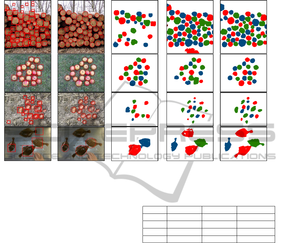
Figure 6: The pictures show some results of our segmentation compared to grab-cut. The first column show the detected
objects marked by rectangles and the second one the verified objects marked by circles. The results of grab-cut are given in
the third column and of our approach with belief-propagation (BP) as well as grab-cut (GC) in the fourth and fifth column.
5.3 Multi-object Segmentation
To evaluate the multi-object segmentation we use the
Huang-Dom-measure (HD-M). The HD-M is based
on the hamming distance from one segmented object
to a corresponding ground truth object and otherwise.
Similar to the f-score, a value of 1 indicates a per-
fect segmentation. Different to the f-score, not seg-
mented objects on a large background can still lead
to a relatively high value, because a not-found corre-
spondence has no penalty in the measure and will be
simply ignored. Consequently, the HD-M is mainly
suitable to compare different methods. The results for
grab-cut, the LSGMC and our GMC-G are presented
in Table 3. The LSGMC separates objects by using
detected objects and a binary image. Our GMC-G im-
proves the LSGMC by combining the separation with
a watershed segmentation. The input binary images
for both methods are generated with graph-cut as de-
scribed before with KD-NN-A or KD-NN-G.
The evaluation results in Table 3 show that our
GMC-G yields for all objects the best results and
Grab-Cut and LSGMC generate in nearly all cases
poorer results. Only in the apple case the grab-cut re-
sults are similar to the GMC-G ones. This is because
the apple detection is nearly perfect. Nevertheless,
grab-cut applied on the verified objects can also fail,
as shown in Figure 6.
Table 3: Evaluation of the multi-object-segmentation with
the HD-Measure. The best values are in bold print.
object grab-cut LSGMC GMC-G
wood 0.89 (0.04) 0.92 (0.15) 0.93 (0.02)
apple 0.99 (0.01) 0.98 (0.01) 0.99 (0.01)
potato 0.95 (0.36) 0.94 (0.03) 0.97 (0.014)
flatfish 0.90 (0.05) 0.83 (0.07) 0.94 (0.03)
6 CONCLUSION
We presented an automatic segmentation method for
organo-groups in images. Such groups consist of or-
ganic objects of similar types (like wood logs, ap-
ples, or tomatoes) on unknown background. Although
approaches for specific objects exist, so far no ap-
proach was general enough to segment such an arbi-
trary group. Although this method needs an object
detector in the first step, the detector does not have
to be very accurate, because the detection results are
verified and the approach can compensate these inac-
curacies.
Our approach generalizes and improves existing
work in combining an object verification method to
optimize the true positive rate, a fore- and background
probability map creation method usable as input for
an optimization based segmentation method, and an
Optimization-basedAutomaticSegmentationofOrganicObjectsofSimilarTypes
597

improved object separation method.
We compare our approach against grab-cut and a
dedicated wood log segmentation method and outper-
form both methods. In the case of wood log segmen-
tation, our approach is even a little bit better than the
dedicated wood log segmentation method.
REFERENCES
Achanta, R., Shaji, A., Smith, K., Lucchi, A., Fua, P., and
S
¨
usstrunk, S. (2012). SLIC Superpixels Compared to
State-of-the-Art Superpixel Methods. Pattern Analy-
sis and Machine Intelligence, IEEE Transactions on,
34(11):2274–2282.
Akin, C., Kirci, M., Gunes, E. O., and Cakir, Y. (2012).
Detection of the pomegranate fruits on tree using
image processing. In Agro-Geoinformatics (Agro-
Geoinformatics), 2012 First International Conference
on, pages 1–4.
Aloisio, C., Mishra, R., Chang, C.-Y., and English, J.
(2012). Next generation image guided citrus fruit
picker. In Technologies for Practical Robot Applica-
tions (TePRA), 2012 IEEE International Conference
on, pages 37 –41.
Boykov, Y. and Kolmogorov, V. (2004). An experimental
comparision of min-cut/max-flow algorithms for en-
ergy minimation in vision. In PAMI, pages 1124–
1137.
Chan, T. F. and Vese, L. A. (2001). Active contours with-
out edges. IEEE Transactions on Image Processing,
10(2):266–277.
Dahl, A. B., Guo, M., and Madsen, K. H. (2006). Scale-
space and watershed segmentation for detection of
wood logs. In Vision Day, Informatics and Mathe-
matical Modelling.
Felzenszwalb, P. F. and Huttenlocher, D. P. (2006). Efficient
belief propagation for early vision. Int. J. Comput.
Vision, 70(1):41–54.
Gutzeit, E., Ohl, S., Kuijper, A., Voskamp, J., and Urban,
B. (2010). Setting graph cut weights for automatic
foreground extraction in wood log images. In VISAPP
2010, pages 60–67.
Gutzeit, E. and Voskamp, J. (2012). Automatic segmen-
tation of wood logs by combining detection and seg-
mentation. In ISVC 2012 - 8th International Sympo-
sium on Visual Computing, volume LNCS 7431, pages
252–261.
Herbon, C., Tnnies, K. D., and Stock, B. (2014). Detection
and segmentation of clustered objects by using iter-
ative classification, segmentation, and gaussian mix-
ture models and application to wood log detection. In
GCPR, pages 354–364.
Huang, Q. and Dom, B. (1995). Quantitative methods of
evaluating image segmentation. In Image Processing,
1995. Proceedings., International Conference on, vol-
ume 3, pages 53 –56 vol.3.
Kass, M., Witkin, A., and Terzopoulos, D. (1988). Snakes:
Active contour models. International Journal of Com-
puter Vision, 1(4):321–331.
Lee, J.-H., Wu, M.-Y., and Guo, Z.-C. (2010). A tank fish
recognition and tracking system using computer vi-
sion techniques. In Computer Science and Informa-
tion Technology (ICCSIT), volume 4, pages 528–532.
Li, S. Z. (1995). Markov random field modeling in computer
vision. Springer-Verlag, London, UK, UK.
Medina Rodriguez, P., Fernandez Garcia, E., and Diaz Ur-
restarazu, A. (1992). Adaptive method for image seg-
mentation based in local feature. Cybernetics and Sys-
tems, 23(3-4):299–312.
Otsu, N. (1979). A threshold selection method from gray-
level histograms. In IEEE Transactions on Systems,
Man and Cybernetics, pages 62–66.
Roth, S. and Black, M. J. (2005). Fields of experts: A
framework for learning image priors. In In CVPR,
pages 860–867.
Rother, C., Kolmogorov, V., and Blake, A. (2004). Grabcut
- interactive forground extraction using iterated graph
cuts. In ACM Transactions on Graphics, pages 309–
314. ACM Press.
Rui, G., Gang, L., and Yongsheng, S. (2010). A recogni-
tion method of apples based on texture features and
em algorithm. In World Automation Congress (WAC),
2010, pages 225 –229.
Sezgin, M. and Sankur, B. (2004). Survey over image
thresholding techniques and quantitative performance
evaluation. Journal of Electronic Imaging, 13(1):146–
168.
Shi, J. and Malik, J. (2000). Normalized cuts and image
segmentation. In IEEE Transactions on Pattern Anal-
ysis and Machine Intelligence, pages 888–905.
Viola, P. A. and Jones, M. J. (2001). Rapid object detection
using a boosted cascade of simple features. In CVPR
(1), pages 511–518.
White, D., Svellingen, C., and Strachan, N. (2006). Auto-
mated measurement of species and length of fish by
computer vision. Fisheries Research, 80(2-3):203–
210.
Wijethunga, P., Samarasinghe, S., Kulasiri, D., and Wood-
head, I. (2008). Digital image analysis based auto-
mated kiwifruit counting technique. In Image and Vi-
sion Computing New Zealand, pages 1 –6.
Zhang, X., Yang, Y.-H., Han, Z., Wang, H., and Gao, C.
(2013). Object class detection: A survey. ACM Com-
put. Surv., 46(1):10:1–10:53.
Zhao, J., Tow, J., and Katupitiya, J. (2005). On-tree fruit
recognition using texture properties and color data. In
Intelligent Robots and Systems, 2005. (IROS 2005).
2005 IEEE/RSJ International Conference on, pages
263 – 268.
Zhu, L.-M., Zhang, Y.-L., Zhang, W., Tao, Z.-C., and Liu,
C.-F. (2012). Fish motion tracking based on rgb color
space and interframe global nerest neighbour. In Auto-
matic Control and Artificial Intelligence (ACAI 2012),
International Conference on, pages 1061–1064.
VISAPP2015-InternationalConferenceonComputerVisionTheoryandApplications
598
