An Interactive Visualization System for Huge Architectural Laser Scans

Thomas Kanzok

, Lars Linsen

and Paul Rosenthal

Department of Computer Science, Technische Universit

at Chemnitz, Chemnitz, Germany

Jacobs University, Bremen, Germany

Keywords:

Point Clouds, Out of Core, Level of Detail, Interactive Rendering.

Abstract:

This paper describes a system for rendering large (billions of points) point clouds using a strict level-of-

detail criterion for managing the data out of core. The system is comprised of an in-core data structure for

managing the coarse hierarchy, an out-of-core structure for managing the actual data and a multithreaded

rendering framework that handles the structure and is responsible for data caching, LOD-calculations, culling,

and rendering. We demonstrate the performance of our approach with two real-world datasets (a 1.8 b points

outdoor scene and a 360 m points indoor scene).

1 INTRODUCTION

Due to the falling prices in the market for 3D scanning

devices, especially for terrestrial laser scanners, it has

become viable for small to middle sized companies to

afford the devices themselves or hire a contractor to

have objects scanned for them. In the ﬁeld of civil en-

gineering in particular a rising popularity of 3D scan-

ning for building documentation can be witnessed at

the moment. However, currently available software

has still not fully solved the problems that arise with

the growth of the produced datasets that can go well

into the gigabytes of binary data.

However, for working with the data not everything

has to be loaded from the disk at once, since parts of

the model will probably not be visible anyways while

other parts are too far away to perceive details. The

key for dealing with this amount of data is to parti-

tion the data conveniently so that invisible parts can

be omitted (culling) while visible parts can be ren-

dered with respect to the actual visible level of detail

(LOD).

Finding an appropriate partitioning of the data that

allows for such algorithms while making best use

of the available hardware, especially the GPUs, has

been an intensively studied ﬁeld since the turn of the

millennium. In recent years the mark of billions of

points has been broken (Elseberg et al., 2013) and the

amounts of data are still rising.

In this paper we present our rendering system for

point clouds that has been tested to work with data

sizes of several billions of points. In order to deal with

this data we had to implement a system that handles

the data out of core, i.e. mostly stored on a hard drive

and only partially resident in RAM or GPU-memory.

Making use of the widespread multicore CPUs we de-

veloped a framework that is able to handle all man-

agement of the structure in parallel without interfer-

ing with the actual interactive rendering. This is not

possible without:

• A space partitioning structure that incorporates hi-

erarchical levels of detail.

• An accurate LOD-estimation scheme.

• A parallel framework that distributes independent

tasks over the available CPU cores.

The paper will mainly give insight into the developed

rendering architecture, but also provide the reader

with enough information to comprehend the under-

lying concepts.

2 RELATED WORK

Investigations of point based rendering have be-

gun long before the widespread use of 3D-scanning

for data acquisition (Levoy and Whitted, 1985),

but gained real drive with the Digital Michelangelo

Project (Levoy, 1999), during which the ﬁrst prac-

tically applicable rendering system for large point

clouds was developed (Rusinkiewicz and Levoy,

2000).

Since then several improvements regarding ren-

dering quality (Botsch and Kobbelt, 2003; Botsch

265

Kanzok T., Linsen L. and Rosenthal P..

An Interactive Visualization System for Huge Architectural Laser Scans.

DOI: 10.5220/0005315202650273

In Proceedings of the 10th International Conference on Computer Graphics Theory and Applications (GRAPP-2015), pages 265-273

ISBN: 978-989-758-087-1

 2015 SCITEPRESS (Science and Technology Publications, Lda.)

et al., 2004; Zwicker et al., 2004) and efﬁciency have

been suggested. Due to the falling prices of increas-

ingly accurate and fast scanning hardware the sizes of

generated datasets have risen drastically and are cur-

rently lying in regions above the billions.

To handle these amounts of data multiple ap-

proaches were published that use different methods to

subdivide the data into a manageable hierarchy (usu-

ally a tree) that allows rendering of hierarchy nodes

with a level-of-detail (LOD) that scales with the ap-

parent size of the node on the screen. This is only

possible if every non-leaf node provides a coarse rep-

resentation of the data that itself and all its children

contain. Previously coarser levels were generated as

the average of ﬁner levels (Rusinkiewicz and Levoy,

2000) but since the publication of Sequential Point

Trees (SPTs) (Dachsbacher et al., 2003) the paradigm

of using ”representative points”, i.e. points that are

a good approximation of a larger set, from ﬁne lay-

ers to create a coarser structure has gained popularity.

Since the original SPTs had to be stored in RAM to be

renderable, they were extended to an out-of-core vari-

ant using nested octrees (Wimmer and Scheiblauer,

2006). Another way to organize points is to handle

them in ”layers” (Gobbetti and Marton, 2004) that

are sorted in a kD-tree manner or to store the data

in the leaves of a kD-tree-like structure (Goswami

et al., 2013) (hence the name ”layered point trees”, or

LPTs). kD-trees have the advantage of allowing for

equally-sized nodes, but have to be reorganized when

changes to the data are made, which is much easier

when using octree-structures.

Although the discussed approaches seem to of-

fer reasonable performance for large datasets they

have certain drawbacks that do not map well to cur-

rent hardware. The SPT-approach is based on a

per-object sorting and therefore does not allow for

culling and ﬁne-grained LOD calculations. This can

be done much better in the LPT-Framework, which is

also nicely suited for GPU rendering. However, the

trees rely on a uniform point distribution, as already

pointed out by the authors, which can not be guaran-

teed in real world scans. Both concerns are addressed

by the nested-octree-approach. However, their er-

ror metric is very coarse and does not account for

ﬂat nodes perpendicular to the viewer, which could

be drawn with considerably fewer points than a cube

that is homogenously ﬁlled with the same amount of

points. Last but not least, most of the mentioned pa-

pers are especially focused on the used data structure

and hardly discuss the rendering framework around it.

This paper shall not only give the reader insights

into the used data management but also explain how

to integrate the data model into a working rendering

framework.

3 GENERAL APPROACH

Our approach makes use of the parallelism of modern

GPUs and CPUs by ofﬂoading all management efforts

to the CPU, leaving the GPU to the task it is best

suited for – rendering. Our main contributions are

a crisp LOD mechanism that includes depth culling

and a parallel out-of-core rendering framework that

allows us to render billions of points in an interactive

way.

The design goal for our data structure was to ﬁnd a

representation of a point cloud that has the following

key features:

1. Out-of-core management of point data, this im-

plies a hierarchical organization.

2. Fine-grained way of selecting a level of detail for

the nodes in the hierarchy.

3. GPU-friendly layout of the hierarchy layers.

The data structure we used to achieve this

goal is inspired by the work of Wimmer and

Scheiblauer (Wimmer and Scheiblauer, 2006). In

contrast to them however, our data is not as tightly

nested in order to allow for batch rendering, as we

will see in the following section. The parallel render-

ing architecture is described in the section after that.

3.1 Data Structure

The data structure of our system is comprised of an

outer structure which is used for calculating a node-

wise LOD and an inner structure which enables the

selection of representative points for the calculated

LOD. The outer structure is designed in a way that al-

lows it to always be completely held in CPU-memory.

It is used for LOD calculation and all implemented

culling mechanisms whereas the inner structure gets

loaded into a vertex buffer object (VBO) from a hard

drive on demand and is used for the actual rendering.

Similar to nested point trees (Wimmer and

Scheiblauer, 2006), our outer structure is an octree

that is used to cut the data into convenient chunks,

each node completely encompassing all of its chil-

dren. The data structure is built top down, starting

with a cubic root node that contains all available data

and is then recursively split into its children while

retaining a number of ”representative points” in the

node.

Those points are chosen using an adaptive n-Tree,

where n is chosen based on the local dimensionality

of the node’s data (see Equation 3.1), meaning the tree

GRAPP2015-InternationalConferenceonComputerGraphicsTheoryandApplications

266

will be binary if the data is distributed along a line,

a quadtree if the data is planar and an octree if the

data spans a volume. The created tree is adaptive in

that it can be given a number of target points to store

and it will keep a homogeneous point distribution by

contracting leaf nodes with higher depth when a node

with lower depth is to be split and the tree would oth-

erwise exceed its capacity. Node capacity will usu-

ally be given by a target GPU buffer size, which will

let every node have either almost the same amount of

points (for uncompressed data) or a number of points

that depends on the compression factor of the node

(see Section 5).

For determining the local dimensionality of a node

we use a criterion introduced by Westin et al. (Westin

et al., 1997), that is an anisotropy value

= c

+ c

+ λ

− 2λ

+ λ

= 1 − c

; (1)

deﬁned by the eigenvalues of λ

, λ

of the covari-

ance matrix of all the points in the node. Here c

, c

and c

; c

= 1 describe the linearity, planarity

and ”sphericality” of the node:

− λ

+ λ

2(λ

− λ

)

+ λ

3λ

+ λ

The values of c

, c

and c

form barycentric coor-

dinates which facilitate a good estimation of planarity

and linearity of a node.

The strict division between structure and data

makes it easy to store the management data of the

whole tree in RAM (for reasonable choices for the

number of points, see Table 1). This will be conve-

nient later for our rendering architecture.

Table 1: The generated number of tree nodes for three target

node sizes (in points per node, ppn) using our test datasets

of 1.8 billion and 367 million points. We assume that node

sizes smaller than 2

= 4096 points are not practical any-

more, since the used VBOs would become much smaller

than 100 kb. The values represent the uncompressed case.

With compression the structure gets smaller.

# points ppn nodes structure size

1.8 billion 2

115498 20.26 MB

56430 9.90 MB

28642 5.03 MB

367 million 2

32120 5.64 MB

11824 2.07 MB

5612 0.98 MB

Nested in the outer structure are abstraction lay-

ers of the point cloud that can essentially be seen as

the layers of Gobbetti and Marton’s Layered Point

Clouds (Gobbetti and Marton, 2004) without the strict

binary balanced subdivision, which we abandoned to

overcome their dependence on homogeneous point

(a) (b) (c)

(d) (e) (f)

(g)

Figure 1: An example for our tree creation process; Each

node holds a reference (shown as a line to the center) to a

representative point, i.e. the point that is currently closest to

the center of the node (a). During tree buildup this reference

can be updated and the tree will be split (b) until the maxi-

mum capacity is reached (10 in this example, (c)). When we

now want to insert a new point ﬁrst the children of the low-

est node are contracted, which propagates the blue point to

the appropriate child in the outer tree. Insertion of the new

node also replaced a representant, making the orange point

also obsolete. The contracted node is marked and may never

be expanded again (bold border) (d). After all points are in-

serted (e) representants for the nodes are sampled homoge-

nously over the data set. A level-order traversal yields the

LOD representation (f), which gets assigned a contour that

takes into account the possible approximation error. The

unused points are inserted into the children of the outer tree

(g).

distribution. We are organizing the points by a

level-order traversal of the previously created adap-

tive n-tree, which enables us to select which points

to render based on their by their ”visual importance”

(see (Dachsbacher et al., 2003)).

Finally the tree nodes get assigned a contour sim-

ilar to the one used by Laine and Karras (Laine and

Karras, 2011). This contour is either the oriented

bounding box of each node with respect to the points

that are stored in the node itself (when the node is

ﬂat enough) or the axis-parallel bounding box of the

node computed during tree construction. We decide

whether a node is ”ﬂat enough” based on the local di-

mensionality (see Equation 3.1). Thresholds of 0.03

AnInteractiveVisualizationSystemforHugeArchitecturalLaserScans

267

(a) Level 3 (b) Level 2

(e) Combined View

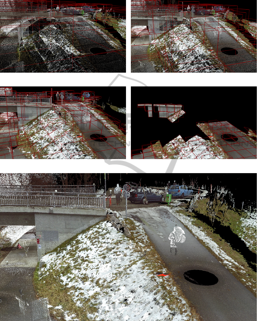
Figure 2: The layer structure of our tree contributes some points from each layer (top) to the ﬁnal rendering (bottom). Note

that some of the bounding volumes are aligned to the geometry, others are not. This is the result of our anisotropy estimator

(Equation 3.1), which allows for a very ﬁne-grained LOD calculation as seen in (d), where nodes on the bridge’s wall are

rendered although parts of the ﬂat hillside perpendicular to the viewer are already left out. (The highest levels 9 to 4 were

omitted for brevity.)

GRAPP2015-InternationalConferenceonComputerGraphicsTheoryandApplications

268

have shown to provide a good distinction, leading to

the classiﬁcation of a node as

Volumetric ⇔ c

> 0.03 or

Planar ⇔ c

> 0.03 or

Linear else

Having computed the contours for each node we

encode them as the principal axes of the node and

store everything to a ﬁle. The amount of stored data

sums up to a maximum of 184 bytes per tree node that

have to be stored in memory. As we can see in Table 1

this should not pose any serious limitation for today’s

computers.

3.2 Rendering Architecture

When rendering our structure we use multiple CPU-

cores to relieve the GPU from any task except the one

it was designed to do best – transforming and raster-

izing primitives. Basically we are using three paral-

lel threads that are working together: an LOD thread

that is responsible for calculating the node’s apparent

size (the level of detail – LOD) and culling invisible

nodes, a loader thread that is responsible for loading

data from the hard drive, and a rendering thread that

takes the visible nodes and their LOD and initiates

rendering of the respective Vertex Buffer Objects (see

Figure 3). This thread is additionally responsible for

mapping and unmapping buffers, since it is the one

that ”owns” the OpenGL context. This approach is

not unlike the one described by Corr

ea et al. (Corr

et al., 2002), but includes a layering- and LOD mech-

anism and is tailored towards optimal buffer usage on

modern GPUs.

3.2.1 Management Structures

The three threads need six core structures in order to

distribute their results among each other. These struc-

tures – which are prone to synchronization issues and

have to be guarded carefully – are:

1. The tree itself and the nodes therein

2. Two rendering lists that store structures necessary

for rendering. One is used for writing into by the

LOD thread (”back”) and one that is read from by

the rendering thread (”front”).

3. A prioritized load queue to which the LOD thread

pushes nodes that have to be loaded and from

which the loader thread pops its appropriate tar-

gets.

4. Two coarse (128×128 pixels) depth buffers, again

one back- and one front buffer for occlusion

culling.

5. A hierarchical node cache that keeps track of a

timestamp for each node that has been used for

actual rendering in order to ﬁnd the least recently

used one for data loading when we have reached

our memory limit.

6. A map queue and an unmap queue for manag-

ing VBOs that are currently mapped for writing

or were recently written by the loader thread and

are now ready for unmapping.

The last two queues have to be managed by the

rendering thread because this thread is associated with

the GL context and therefore the only one that can

issue GL commands for mapping and unmapping of

buffer memory (Hrabcak and Masserann, 2012).

3.2.2 LOD Thread

The LOD thread is responsible for maintaining a list

of visible nodes that can be read by the rendering

thread to draw the respective Buffer Objects. While

the software is running this thread goes through the

hierarchy repeatedly and calculates the projected size

of a node’s contour on the screen. In order to do this

as strictly as possible we are transforming the con-

tour of each node to screen coordinates in software

while performing frustum culling. Additionally we

are using our coarse depth buffer to perform occlu-

sion culling. The depth test is done by rasterizing the

node’s contours in software using a parallel coverage-

based rasterizer similar to (Pineda, 1988). We decided

against a hardware-based occlusion culling (Bittner

et al., 2004) because we wanted to unload the GPU

from any tasks except rendering and we assume that

current and coming CPUs will have enough cores

to accomplish this task. For each node that passes

through these stages we can calculate its projected

size on the screen and use this value as the LOD for

this node.

We now have to check whether the node’s data is

already loaded from the HDD, in which case we can

append its required rendering data (VBO Id, LOD, in-

ternal GL type) to the rendering queue. If no data is

loaded yet for this node we calculate a priority value

based on the distance of the node from the viewer (to

start ﬁlling the space close to the viewer) and push the

node to the load queue.

When the LOD thread has ﬁnished the two ren-

dering lists and the two depth buffers are swapped the

thread begins anew from the root node. Care has to

be taken to avoid synchronization issues with the re-

sources shared between the threads, a schematic im-

age of the whole architecture including the necessary

locks can be found in Figure 3.

AnInteractiveVisualizationSystemforHugeArchitecturalLaserScans

269

read

write

Front

Back

Switch

Rendering Queues

read

write

Front

Back

Switch

Depth Buffers

Load QueueNode Cache

Mapped Queue

Unmap Queue

Tree

LOD Thread

Rendering Thread

Loader Thread

traverse tree

take node

calculate LOD

write

swap

update

read

write

swap

push

lock

render

unlock

take LRU

map data

push

take first

unmap

take first

push

take first

load data

read

verify

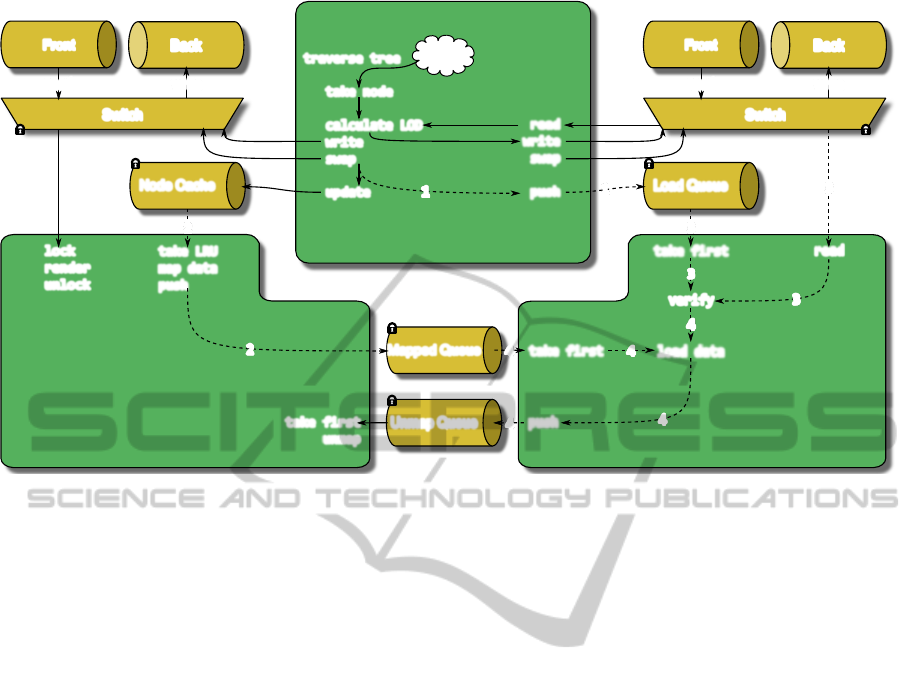
Figure 3: Overview of the data structures used by our rendering architecture. Detailed descriptions of the behavior of the

threads can be found in the respective sections. The dashed parts are only carried out when their respective conditions are

met: (1) A node is visible but not loaded (2) The mapped queue is not full (3) The load queue is not empty (4) The node is

still visible.

3.2.3 Loader Thread

Whenever the load queue is not empty the loader

thread takes the top node from the load queue, re-

moves it from the queue and again performs the oc-

clusion and frustum checks allready described for the

LOD thread. This avoids unnecessary HDD accesses

to load nodes that are not even visible anymore be-

cause the user has lost them from his view in the

meantime. If the node is still visible the thread gets

a pointer to mapped memory from the list of mapped

buffers and loads the data into the buffer (This ap-

proach is inspired by Hrabcak and Masseran’s inves-

tigations on asynchronous buffer transfers (Hrabcak

and Masserann, 2012)). When this is done it pushes

the node to the rendering threads unmap queue and

tries to read the next node.

3.2.4 Rendering Thread

This thread is responsible for displaying the data in

the given LOD. The front rendering list that was pre-

viously ﬁlled by the LOD thread is now processed by

issuing a draw call for each VBO in the list. Prior to

that the thread has also to take care of unmapping all

recently loaded nodes from the mapped queue and of

assuring that the map queue is ﬁlled with pointers to

memory usable for the loader thread.

Currently, the two queues have a ﬁxed size of 5

buffers. In order to keep the mapped queue ﬁlled the

rendering thread requests up to 5 recently used nodes

from the cache, maps their associated buffers to RAM

and marks the nodes as ”not loaded”. Based on our

experiments we concluded that a cache size of 2000

nodes sufﬁces to have all visible nodes loaded and still

have a reserve to map. This is of course dependent on

the number of points stored per node and will proba-

bly not be enough when sizes smaller than in Table 3

are used, but we do not think that using yet smaller

nodes would be beneﬁcial under any circumstances.

The actual rendering in our system uses a color-

and a geometry-buffer as described by Saito et

al. (Saito and Takahashi, 1990) to enable deferred

shading and to estimate the necessary normals in

image space, should none be given in the data.

Optionally we support a splatting approach similar

to (Preiner et al., 2012) to even out illumination in-

consistencies between different scans (Kanzok et al.,

2012).

3.2.5 Load Distribution

The LOD thread may not be much slower than the

rendering thread in order to keep up with the render-

ing. Since we are targeting at least 10 fps for our

application to be considered ”interactive” we have a

time of 100 ms available each frame for one run of

the threads.

GRAPP2015-InternationalConferenceonComputerGraphicsTheoryandApplications

270

Table 2: The measured timings for different conﬁgurations

of visible nodes and visible points. As one can see the tim-

ings are sufﬁcient for interactive rendering, however, the

bottleneck is the streaming of points from the HDD to the

GPU (see Section 4).

nodes points LOD (ms) Rendering (ms)

293 6.6 m 3.6 52.2

726 10.4 m 18.0 63.8

472 10.4 m 7.3 58.5

138 5.7 m 3.5 52.5

350 11.5 m 18.0 68.8

250 13.1 m 7.0 56.2

64 65.5 m 3.9 66.4

166 13.8 m 13.3 72.0

166 18.3 m 4.7 50.6

We can see in Table 2 that this aim can be achieved

in most conﬁgurations. The loader thread is not criti-

cal in this respect since it only ever takes one node,

loads it and signals it back to the rendering thread

which in turn unmaps the buffer and renders the node.

This achieves an implicit synchronization between the

two threads, at least at a per-node level.

4 RESULTS & DISCUSSION

The choice for the number of representants k of a

node has severe implications for VBO-size, manage-

ment overhead, and streaming efﬁciency. We used

two datasets to investigate the effects of node sizes on

these factors, both generated by laser scanning real

world scenes: one outdoor scene of a bridge with

slightly over 1.8 b points and one indoor scene of a

small ofﬁce with just above 360 m points. While the

indoor scene had lots of occlusion due to multiple

walls it was considerably smaller. The outdoor scene

on the other hand had extremely dense areas (see e.g.

Figure 4c) but much less occlusion. The experiments

were carried out on a workstation PC with an Intel

Core i7 CPU running Windows 7 64bit and a GeForce

GTX 680 GPU with 2048MB DDR5 memory.

We carried out different experiments to determine

the optimal node size and the best VBO usage strat-

egy in terms of loading and rendering speed. To as-

sure that no caching effects of the operating system or

the hard drive would skew the results we made sure

that no dataset was used twice in succession. The

timings taken for the frames per second were aver-

aged over 5 seconds for each view. The views were

chosen with respect to typical applications. For the

outdoor scene we have one overview over the whole

scene, one closeup view as it could occur when ﬂying

through the data or measuring and one detail view that

makes full use of the detail level in the data. Similarly

the views for the ofﬁce were chosen (Figure 4).

The experiments, summarized in Table 3, have

shown that neither the LOD-calculation including

software-rasterization for the occlusion test nor the

actual rendering speed are seriously limiting the in-

teractivity of the application.

With a worst case of eight frames per second ren-

dering speed we are always able to navigate the scene

without very noticeable stuttering, especially since

the drop in framerate only occurred when viewing ex-

tremely dense areas as seen in Figure 4c. At the mo-

ment the only issue is the time necessary to stream

new data from the harddrive to the GPU. However,

since rendering and interaction are not bound to the

speed of the loader thread, navigating the scene al-

ways stays possible and thanks to the layered struc-

ture of our data the user always has enough informa-

tion about his environment to keep working with the

data.

In terms of the most efﬁcient node (and accord-

ingly VBO) sizes we can draw the following conclu-

sions from our experiments:

1. More points per node lead to less visible nodes

in the scene and to slightly shorter loading times.

This comes at the price of more points that have

to be drawn in each frame, because the coarser

the structure gets, the more difﬁcult it becomes to

calculate a precise LOD for a node.

2. Fewer points per node allow for a more precise

LOD-calculation which leads to higher fps. How-

ever, the number of visible nodes can get very

high which has to be taken into account when de-

signing the cache.

As it is we tend to prefer the medium size of 65536

points per node. At this size our binary point data

amounts to exactly 1.5 MB per node, which ﬁts nicely

into a VBO and it seems to offer the best compromise

between loading and rendering speed.

5 CONCLUSIONS

We have presented an out of core rendering frame-

work for large point models that efﬁciently distributes

the main tasks over the cores of the CPU. The GPU

is therefore free to handle the actual rendering of the

points. Experiments with two real world datasets have

shown the capability of the system to cope with huge

a amount of data. A remaining issue is the optimiza-

tion of streaming efﬁciency from HDD to GPU. This

could be mitigated by compressing the data in the fol-

lowing form:

AnInteractiveVisualizationSystemforHugeArchitecturalLaserScans

271

(a) Overview (b) Close View (c) Detail View

(d) Overview (e) Close View (f) Detail View

Figure 4: The three views in each two datasets used for the comparison in Table 3. The bridge was viewed from far and near

above (a and b) and from below (c). The ofﬁce was viewed from above (a), from the entrance (b) and on an actual desk inside

(c). Navigation from one point to another can happen smoothly and without stalling due to the external handling of node

loading and LOD-calculation.

Table 3: The table shows the number of nodes and points that are rendered for the respective views as well as the times taken

until the view was completely loaded (under the transition-arrows). The node sizes used where 32768, 65536 and 131072

points per node (ppn). The worst conﬁgurations are emphasized in bold.

ppn # visible Overview loading Close View loading Detail View

nodes points fps → nodes points fps → nodes points fps

with z-test 294 6.7 m 19 11.8 s 923 17.7 m 14 4.9 s 452 11.8 m 17

w/o z-test 298 6.7 m 19 19.0 s 1304 22.5 m 11 4.8 s 481 12.7 m 16

with z-test 183 7.8 m 15 7.6 s 469 19.6 m 13 3.4 s 235 14.0 m 24

w/o z-test 197 8.0 m 16 11.9 s 661 25.3 m 10 3.8 s 261 15.5 m 15

with z-test 89 9.1 m 10 7.4 s 257 21.8 m 12 3.9 s 161 18.6 m 14

w/o z-test 89 9.1 m 12 11.6 s 388 30.0 m 10 4.7 s 175 20.2 m 13

with z-test 26 736 k 56 8.1 s 846 18.7 m 16 0.9 s 107 3.5 m 49

w/o z-test 26 764 k 56 33.0 s 1910 36.7 m 8 0.6 s 109 3.5 m 57

with z-test 19 1.0 m 54 7.0 s 452 23.3 m 16 1.1 s 79 5.1 m 51

w/o z-test 20 1.0 k 55 19.1 s 998 41.8 m 8 1.1 s 81 5.3 m 55

with z-test 22 631 k 57 10.9 s 798 20.5 m 18 0.8 s 53 1.7 m 58

w/o z-test 23 736 k 57 17.5 s 1106 26.4 m 15 0.8 s 57 1.8 m 57

Positions could be encoded as unsigned

integer coordinates corresponding to the

OpenGL data types GL UINT, GL USHORT,

GL UNSIGNED INT 2 10 10 10 REV and GL UBYTE,

making it possible to use 96, 48, 32 or 24 bits per

position. This does not reach the high compression

factors demonstrated by other researchers (e.g. (Chou

and Meng, 2002)), but lets us do the decompression

in specialized GPU hardware with nearly no overhead

and does not need connectivity information. Each

node stores the minimum of its octree-bounding

box o and a sampling resolution r that get passed

to the vertex shader as uniform, which will then

compute compute the actual vertex position x from

the compressed one

x as follows:

x = o +

x ◦ r, (2)

with ◦ denoting a component-wise multiplication.

The quantiﬁcation of colours could be achieved

for example by simultaneously building a Kohonen

map (Boggess et al., 1994) from the point colours dur-

ing structure buildup, the normals can be quantised

according to a uniform distribution on the unit sphere.

This can be achieved by applying several Lloyd-

relaxations (Lloyd, 1982) to an energy-minimizing

pattern (Rakhmanov et al., 1994). According to our

calculations this could reduce the data size to

which would hopefully translate to the loading times

as well.

GRAPP2015-InternationalConferenceonComputerGraphicsTheoryandApplications

272

Due to the hierarchical structure changes in data

size do not pose a problem for our approach. Pro-

cessing fewer points may improve performance, since

more points will ﬁt in the cache minimizing loading

effort. Using more points will result in longer pre-

processing (O(n log n) due to the tree buildup), but

rendering performance should not be affected.

ACKNOWLEDGEMENTS

The authors would like to thank the enertec engineer-

ing AG (Winterthur, Switzerland) for providing us

with the data and for their close collaboration. This

work was partially funded by EUREKA Eurostars

(Project E!7001 ”enercloud - Instantaneous Visual In-

spection of High-resolution Engineering Construction

Scans”).

REFERENCES

Bittner, J., Wimmer, M., Piringer, H., and Purgathofer, W.

(2004). Coherent hierarchical culling: Hardware oc-

clusion queries made useful. Computer Graphics Fo-

rum, 23(3):615–624.

Boggess, J.E., I., Nation, P., and Harmon, M. (1994). Com-

pression of color information in digitized images us-

ing an artiﬁcial neural network. In Proc of NAECON,

pages 772–778 vol.2.

Botsch, M. and Kobbelt, L. (2003). High-quality point-

based rendering on modern GPUs. In Proc. on Paciﬁc

Graphics, pages 335–343.

Botsch, M., Spernat, M., and Kobbelt, L. (2004). Phong

splatting. In Proc. of SPBG, pages 25–32.

Chou, P. and Meng, T. (2002). Vertex data compression

through vector quantization. IEEE Trans. Vis. & Com-

put. Graph., 8(4):373–382.

Corr

ea, W. T., Klosowski, J. T., and Silva, C. T. (2002).

iwalk: Interactive out-of-core rendering of large mod-

els. Technical report, Technical Report TR-653-02,

Princeton University.

Dachsbacher, C., Vogelgsang, C., and Stamminger, M.

(2003). Sequential point trees. In Proc. of SIG-

GRAPH, SIGGRAPH ’03, pages 657–662, New York,

NY, USA. ACM.

Elseberg, J., Borrmann, D., and N

uchter, A. (2013). One

billion points in the cloud an octree for efﬁcient pro-

cessing of 3d laser scans. Journal of Photogrammetry

and Remote Sensing, 76(0):76 – 88.

Gobbetti, E. and Marton, F. (2004). Layered point clouds.

In Proc. of SPBG, SPBG’04, pages 113–120, Aire-la-

Ville, Switzerland, Switzerland. Eurographics Associ-

ation.

Goswami, P., Erol, F., Mukhi, R., Pajarola, R., and Gob-

betti, E. (2013). An efﬁcient multi-resolution frame-

work for high quality interactive rendering of massive

point clouds using multi-way kd-trees. The Visual

Computer, 29(1):69–83.

Hrabcak, L. and Masserann, A. (2012). Asynchronous

buffer transfers. In Cozzi, P. and Riccio, C., edi-

tors, OpenGL Insights, pages 391–414. CRC Press.

http://www.openglinsights.com/.

Kanzok, T., Linsen, L., and Rosenthal, P. (2012). On-the-

ﬂy Luminance Correction for Rendering of Inconsis-

tently Lit Point Clouds. Journal of WSCG, 20(2):161

– 169.

Laine, S. and Karras, T. (2011). Efﬁcient sparse voxel oc-

trees. IEEE Trans. Vis. & Comp. Graph., 17(8):1048–

1059.

Levoy, M. (1999). The digital michelangelo project. In

Proc. on 3-D Digital Imaging and Modeling, pages 2–

11.

Levoy, M. and Whitted, T. (1985). The use of points as

a display primitive. Technical report, University of

North Carolina, Department of Computer Science.

Lloyd, S. (1982). Least squares quantization in pcm. IEEE

Trans. Inform. Theory, 28(2):129–137.

Pineda, J. (1988). A parallel algorithm for polygon ras-

terization. In Proc. of SIGGRAPH, SIGGRAPH ’88,

pages 17–20, New York, NY, USA. ACM.

Preiner, R., Jeschke, S., and Wimmer, M. (2012). Auto

splats: Dynamic point cloud visualization on the

GPU. In Proc. of EGPGV, pages 139–148.

Rakhmanov, E., Saff, E., and Zhou, Y. (1994). Minimal dis-

crete energy on the sphere. Math. Res. Lett, 1(6):647–

662.

Rusinkiewicz, S. and Levoy, M. (2000). Qsplat: A mul-

tiresolution point rendering system for large meshes.

In Proc. of SIGGRAPH, SIGGRAPH ’00, pages 343–

352, New York, NY, USA. ACM Press/Addison-

Wesley Publishing Co.

Saito, T. and Takahashi, T. (1990). Comprehensible ren-

dering of 3-d shapes. SIGGRAPH Comput. Graph.,

24(4):197–206.

Westin, C.-F., Peled, S., Gudbjartsson, H., Kikinis, R., and

Jolesz, F. A. (1997). Geometrical diffusion measures

for MRI from tensor basis analysis. In ISMRM ’97,

page 1742, Vancouver Canada.

Wimmer, M. and Scheiblauer, C. (2006). Instant points:

Fast rendering of unprocessed point clouds. In Proc.

of SPBG, SPBG’06, pages 129–137, Aire-la-Ville,

Switzerland, Switzerland. Eurographics Association.

Zwicker, M., R

anen, J., Botsch, M., Dachsbacher, C.,

and Pauly, M. (2004). Perspective accurate splatting.

In Proc. of Graphics Interface, GI ’04, pages 247–

254, School of Computer Science, University of Wa-

terloo, Waterloo, Ontario, Canada. Canadian Human-

Computer Communications Society.

AnInteractiveVisualizationSystemforHugeArchitecturalLaserScans

273