
Improving the Egomotion Estimation by Correcting the Calibration Bias
Ivan Kre
ˇ
so and Sini
ˇ
sa
ˇ
Segvi
´
c
University of Zagreb Faculty of Electrical Engineering and Computing, Unska 3, 10000 Zagreb, Croatia
Keywords:
Stereo Vision, Camera Motion Estimation, Visual Odometry, Feature Tracking, Camera Calibration, Camera
Model Bias, Deformation Field.
Abstract:
We present a novel approach for improving the accuracy of the egomotion recovered from rectified stereo-
scopic video. The main idea of the proposed approach is to correct the camera calibration by exploiting the
known groundtruth motion. The correction is described by a discrete deformation field over a rectangular
superpixel lattice covering the whole image. The deformation field is recovered by optimizing the reprojec-
tion error of point feature correspondences in neighboring stereo frames under the groundtruth motion. We
evaluate the proposed approach by performing leave one out evaluation experiments on a collection of KITTI
sequences with common calibration parameters, by comparing the accuracy of stereoscopic visual odometry
with original and corrected calibration parameters. The results suggest a clear and significant advantage of the
proposed approach. Our best algorithm outperforms all other approaches based on two-frame correspondences
on the KITTI odometry benchmark.
1 INTRODUCTION
Egomotion estimation is a technique which recov-
ers the camera displacement from image correspon-
dences. The technique is important since it can pro-
vide useful initial solution for more involved struc-
ture and motion (SaM) estimation approaches, which
perform partial or full 3D reconstruction of the scene
(Vogel et al., 2014). These approaches are appeal-
ing due to many potential applications in robotic (e.g.
autonomous navigation (Diosi et al., 2011)) and au-
tomotive systems (e.g. driver assistance (Nedevschi
et al., 2013) and road safety inspection).
Visual odometry (Nist
´
er et al., 2004) is an interest-
ing special case of egomotion estimation, where we
wish to recover the camera trajectory over extended
navigation essays with predominantly forward mo-
tion. In this special case, complex techniques such
as batch reconstruction (global bundle adjustment) or
recognizing previously visited places (loop closing)
are inapplicable due to huge computational complex-
ity involved and/or real time requirements. Hence,
the only remaining option is to recover partial camera
displacements over short sequences of input frames
and to build the overall trajectory by patching them
one after another. The resulting techniques are neces-
sarily prone to the accumulation of incremental error,
just as the classical wheel odometry, and are hence
collectively denoted as visual odometry.
Due to conceptual simplicity and better stability,
the camera egomotion is usually recovered in cali-
brated camera setups. Camera calibration is the pro-
cess of estimating the parameters of a camera model
which approximates the image formation. When we
have a calibrated camera, we can map every image
pixel to a 3D ray emerging from the focal point of
the camera and spreading out to the physical world.
Most perspective cameras can be calibrated reason-
ably well by parametric models which extend the
pinhole camera with radial and tangential distortion.
However, there is no guarantee that this model has
enough capacity to capture all possible distortions of
real camera systems in enough detail, especially when
high reconstruction accuracy is desired. For exam-
ple, many popular calibration models assume that the
distortion center coincides with the principal point
(Zhang, 2000), while it has been shown that this does
not hold in real cameras (Hartley and Kang, 2005). A
good overview of the camera calibration techniques
and different camera models is given in (Sturm et al.,
2011).
In this paper, we propose a novel approach for cor-
recting the calibration of a stereoscopic camera sys-
tem. In our experiments we come to the conclusion
that the reprojection error is not uniformly distributed
across the stereo image pair and that there exists a reg-
347
Krešo I. and Šegvi
´
c S..
Improving the Egomotion Estimation by Correcting the Calibration Bias.
DOI: 10.5220/0005316103470356
In Proceedings of the 10th International Conference on Computer Vision Theory and Applications (VISAPP-2015), pages 347-356
ISBN: 978-989-758-091-8
Copyright
c
2015 SCITEPRESS (Science and Technology Publications, Lda.)

ularity in the reprojection error bias. We hypothesize
that this disturbance in the reprojection error distribu-
tion is caused by inaccurate calibration due to insuf-
ficient capacity of the assumed distortion model. We
propose to alleviate the disturbance by a local cam-
era model (Sturm et al., 2011) formulated as a de-
formation field over a rectangular superpixel lattice
in the two images of stereo pair. The proposed cam-
era model has many parameters and hence requires a
large amount of training data. Thus we propose to
learn the parameters of our deformation field by ex-
ploiting the groundtruth camera motion and point fea-
ture correspondences in neighboring frames. The two
principal contributions of this paper are as follows:
• a statistical analysis of the reprojection error by
utilizing the groundtruth motion (subsection 4.2);
• a technique for correcting the camera calibration
by exploiting the groundtruth motion for learning
the image deformation field (subsection 4.3).
The experimental results presented in Section 5
show that the proposed approach is able to signifi-
cantly improve the accuracy of the recovered camera
motion. Our best algorithm outperforms all other ap-
proaches based on two-frame correspondences on the
KITTI odometry benchmark.
2 RELATED WORK
An increasing number of papers focusing on visual
odometry is an evidence of the problem importance.
A detailed overview of the field can be found in
(Scaramuzza and Fraundorfer, 2011; Fraundorfer and
Scaramuzza, 2012). Most recent implementations are
based on the approach that was proposed in (Nist
´
er
et al., 2004). The main contribution of their approach
is that they did not define the cost function as a so-
lution to point alignment problem in 3D space like
earlier researchers (Moravec, 1980; Moravec, 1981).
Instead, they used the 3D-to-2D cost function which
minimizes the alignment error in 2D image space
popularly called the reprojection error. The advantage
of defining the error in image space is that it avoids the
problem of triangulation uncertainty on the depth axis
where the error variance is much larger compared to
other two axes.
Most of the recent work is focused on constraining
the optimization with multi-frame feature correspon-
dences to achieve better global consistency (Badino
et al., 2013; Konolige and Agrawal, 2008), by ex-
perimenting with new feature detectors and descrip-
tors (Konolige et al., 2007) or by doing a further re-
search in feature tracking and outlier rejection tech-
niques (Badino and Kanade, 2011; Howard, 2008).
Despite the vast amount of research on visual odom-
etry done so far, we did not stumble upon any work
addressing the impact of calibration to the accuracy
of the results nor approaches to improve the calibra-
tion by employing the groundtruth motion data. We
have previously shown (Kreso et al., 2013) that the
accuracy of the reconstructed motion significantly de-
pends on the quality of the calibration target (A4 pa-
per vs LCD monitor). Now we go a step further by
proposing a method for correcting the calibration bias
due to insufficient capacity of the camera model.
3 STEREOSOPIC VISUAL
ODOMETRY
A typical visual odometry pipeline is illustrated in
Figure 1. Acquired images are given to the feature
tracking process where the features are detected and
descriptors extracted. The descriptors are then used to
find the correspondent features in temporal (two adja-
cent frames) and spatial (stereo left and right) domain.
Temporal and stereo matching can be performed inde-
pendently if we do not apply feature detector in right
images, or jointly if we do. After the feature matching
the correspondences typically contain outliers which
are usually rejected by random sampling. Finally we
can optimize an appropriate cost function to recover
the camera motion. Note that the image acquisition
block in Figure 1 also contains the image rectification
procedure which depends on camera calibration.
FEATURE
DETECTION
AND
DESCRIPTOR
EXTRACTION
IMAGE
ACQUISITION
TEMPORAL
MATCHING
STEREO
MATCHING
OUTLIER
REJECTION
MOTION
ESTIMATION
Figure 1: A typical visual odometry pipeline.
3.1 Feature Tracking
In order to recover the camera motion we must
first find enough point correspondences between two
stereo image pairs. It is assumed that the stereo rig
is calibrated and that the images are rectified (their
acquisition is described by a rectified stereo cam-
era model). We use a similar tracking technique as
(Nist
´
er et al., 2004) and (Badino et al., 2013). We de-
tect Harris point features (Harris and Stephens, 1988)
only in left images and perform brute-force matching
of their descriptors inside a search window to obtain
left camera monocular tracks. To extract the descrip-
tors we simply crop plain patches of size 15x15 pix-
els around each detected corner. We establish corre-
VISAPP2015-InternationalConferenceonComputerVisionTheoryandApplications
348

spondences based on the normalized cross-correlation
metric (NCC) between pairs of point features. In or-
der to reduce the localization drift in tracking, we
match all features in the current frame to the oldest
occurrences.
To obtain the full stereo correspondences, we
measure the disparity of every accepted left monoc-
ular track by searching for the best correspondence in
the right image along the same horizontal row. Here
again we compare the plain patch descriptors with
NCC. Compared with matching of independently de-
tected point features, this approach is more robust
to poor repeatability at the price of somewhat larger
computational complexity.
3.2 Cost Function Formulation
Let us denote an image point as q = (u, v)
>
. Now
we can define the points q
k
i,t−1
in the previous frame
(t −1) and q
k
i,t
in the current frame (t), where i ∈ [1, N]
is the index of the point and k ∈ {l, r} is the value
denoting if the point belongs to the left or right image.
Let us subsequently denote X
i,t
as the i-th 3D point in
the current frame (t):
X
i,t
= (x, y, z)
>
= t
t
t(q
l
i,t
, q
r
i,t
) , (1)
where t
t
t() is the function which triangulates the 3D
point in world coordinate system from measured left
and right image points. The goal of egomotion esti-
mation is to recover the 3x3 rotation matrix R and the
3x1 translation vector t that satisfy the 6DOF rigid
body motion of the tracked points.
In order to formulate the cost function we first
need a camera model to describe the image acquisi-
tion process by connecting each image pixel with the
corresponding real world light ray falling on the cam-
era sensor. This can be done using perspective projec-
tion with addition of nonlinear lens distortion model.
For brevity, we skip the modeling of lens distortion
and stereo rectification and assume that the images are
already rectified. The following equation introduces
the pinhole camera model which uses the perspective
projection π to project the world point X = (x, y, z)
>
to the point q = (u, v)
>
on the image plane.
λ
u
v
1
= π(X, R, t) =
f 0 c
u
0 f c
v
0 0 1
[R|t]
x
y
z
1
(2)
The first part is the camera matrix containing the in-
trinsic camera parameters f , c
u
and c
v
. The distance
of the focal point from the image plane f does not cor-
respond directly to the focal length of the lens, since
it also depends on the type and distance of the cam-
era sensor. The principal point (c
u
, c
v
) is the image
location where the z-axis intersects the image plane.
Now we can formulate the cost function for the
two-frame egomotion estimation as a least squares
optimization problem with the error defined in the im-
age space:
argmin
R,t
N
∑
i=1
{l,r}
∑
k
kq
k
i,t
− π(X
i,t−1
, R, t
k
)k
2
(3)
t
l
= t, t
r
= t
l
− (b, 0, 0)
>
(4)
The cost function described by equation (3) is known
as the reprojection error. To minimize the reprojec-
tion error, an iterative non-linear least squares opti-
mization like first order Gauss-Newton (Geiger et al.,
2011) or second order Newton method (Badino and
Kanade, 2011) is usually employed. The equation (3)
shows that we are searching for a motion transforma-
tion which will minimize the deviations between im-
age points measured in the current frame and the re-
projections of the transformed 3D points triangulated
in the previous frame. The motion transformation is
represented by the matrix [R|t] which captures the
motion of 3D points with respect to the static cam-
era. We obtain the camera motion with respect to
the world by simply taking the inverse transformation
[R|t]
−1
. One nice property of the transformation ma-
trix emerging from the orthogonality of rotation ma-
trices is that the inverse transformation is fast and easy
to compute as shown in equation (5).
[R|t]
−1
=
R t
0
>
1
−1
=
R
>
−R
>
t
0
>
1
(5)
Note that the optimization is performed with re-
spect to six free parameters, three describing the cam-
era rotation matrix R and three describing the transla-
tion vector t. The equation (4) describes the relation-
ship between translations of the left and right cameras
in the rectified stereo case. This is because the X
i
is
triangulated in coordinate system of the left camera
and we need to shift it along x axis for the baseline
distance b in the case when we are projecting to the
right camera image plane. Note that the rotation ma-
trix is the same for the left and right cameras because
after the rectification they are aligned to have coplanar
image planes and they share the same x-axis. Because
the baseline b is estimated in the camera calibration
and rectification steps the number of free parameters
for translation remains three.
ImprovingtheEgomotionEstimationbyCorrectingtheCalibrationBias
349

4 LEARNING AND CORRECTING
THE CALIBRATION BIAS
In our previous research we have studied the influ-
ence of subpixel correspondence and online bundle
adjustment to the accuracy of the camera motion esti-
mated from rectified stereoscopic video. Our prelim-
inary experiments have pointed out a clear advantage
of these techniques in terms of translational and rota-
tional accuracy on the artificial Tsukuba stereo dataset
(Martull et al., 2012). However, to our surprise, this
impact was significantly weaker on the KITTI dataset
(Geiger et al., 2012; Geiger et al., 2013). Therefore,
we have decided to investigate this effect by observ-
ing the reprojection error of two-frame point-feature
correspondences under the KITTI groundtruth cam-
era motion which was measured by an IMU-enabled
GPS device.
4.1 Analysis of the Feature
Correspondences
The analysis pointed out many perfect correspon-
dences with large reprojection errors under the
groundtruth camera motion. Figure 2 shows some
examples of this effect where the points and the im-
age patches describing them are displayed. If we look
closely to any of the four patches, we can conclude
that the localization error between any of the four
frames should be less than 1 pixel. However, the re-
projection errors evaluated for the groundtruth motion
(cf. Table 1) are much larger than the localization er-
rors (7 pixel vs 1 pixel). After observing this we won-
dered whether this is a property of a few outliers or
whether there is a regularity with respect to the image
location.
4.2 Statistical Analysis of the
Reprojection Error
After observing many perfect correspondences with
large reprojection errors we decided to verify whether
this effect depends on image location. We divide the
image space into a lattice of superpixel cells in which
we accumulate the reprojection error vectors. Note
that for every stereo correspondence containing 4 fea-
ture points we have two reprojection errors, one in
the left image and the other in the right image. A sin-
gle left or right reprojection error is defined by three
feature points which can be observed in equation (3).
Now for each reprojection error we share the respon-
sibility between the three points equally, by dividing
the vector by 3 and adding it to the cells containing
Table 1: Reprojection errors of the selected correspon-
dences from Figure 2 evaluated for the groundtruth motion.
The errors have much larger values than the uncertainty of
the point feature locations, as seen in Figure 2.
Color Left error Right error
Red 7.10 7.01
Green 6.68 6.56
Blue 7.4 7.32
Yellow 6.75 6.35
the three points responsible for that error. Figure 3
shows the obtained distribution of the reprojection er-
ror vectors for left camera image in each cell. We
computed the means of the error vector L2 norms and
means and variances on the two image axes spanning
the 2D error vector space. Additionally we used norm
means to draw the heat map of the reprojection error
distribution across the image.
By looking at the heat map and the means in Fig-
ure 3(c) we can conclude that the error minimum is
close to the image center and that the error increases
as we move away from the image center. Even more
importantly, we can observe that the vector means
given in Figure 3(d-e) are biased in certain directions
and that this bias is significant considering the error
variances given in Figure 3(f-g). Figure 3 shows that
the minimal error of the camera model appears to be
slightly displaced from the principal point of the im-
age which is very close to the image center. This dis-
placement may be showing us that the center of the ra-
dial distortion is not in the principal point of the cam-
era as assumed by the employed rectification model.
This problem was already observed in (Hartley and
Kang, 2005) where the authors proposed a method for
estimating the radial distortion center.
To confirm that these effects are not due to
some strange bias within the tracker, we performed
the same statistical analysis on the Tsukuba stereo
dataset. Figure 4 shows the same heat map as
we showed before. However, we see that here,
on Tsukuba, the reprojection error is uniformly dis-
tributed without any observable pattern. Note that
the contrast between cells is large due to histogram
equalization but the actual values are distributed in
the range from 0.16 to 0.18. Here we didn’t show that
the error vector means on u and v axes are zero, for
brevity.
VISAPP2015-InternationalConferenceonComputerVisionTheoryandApplications
350
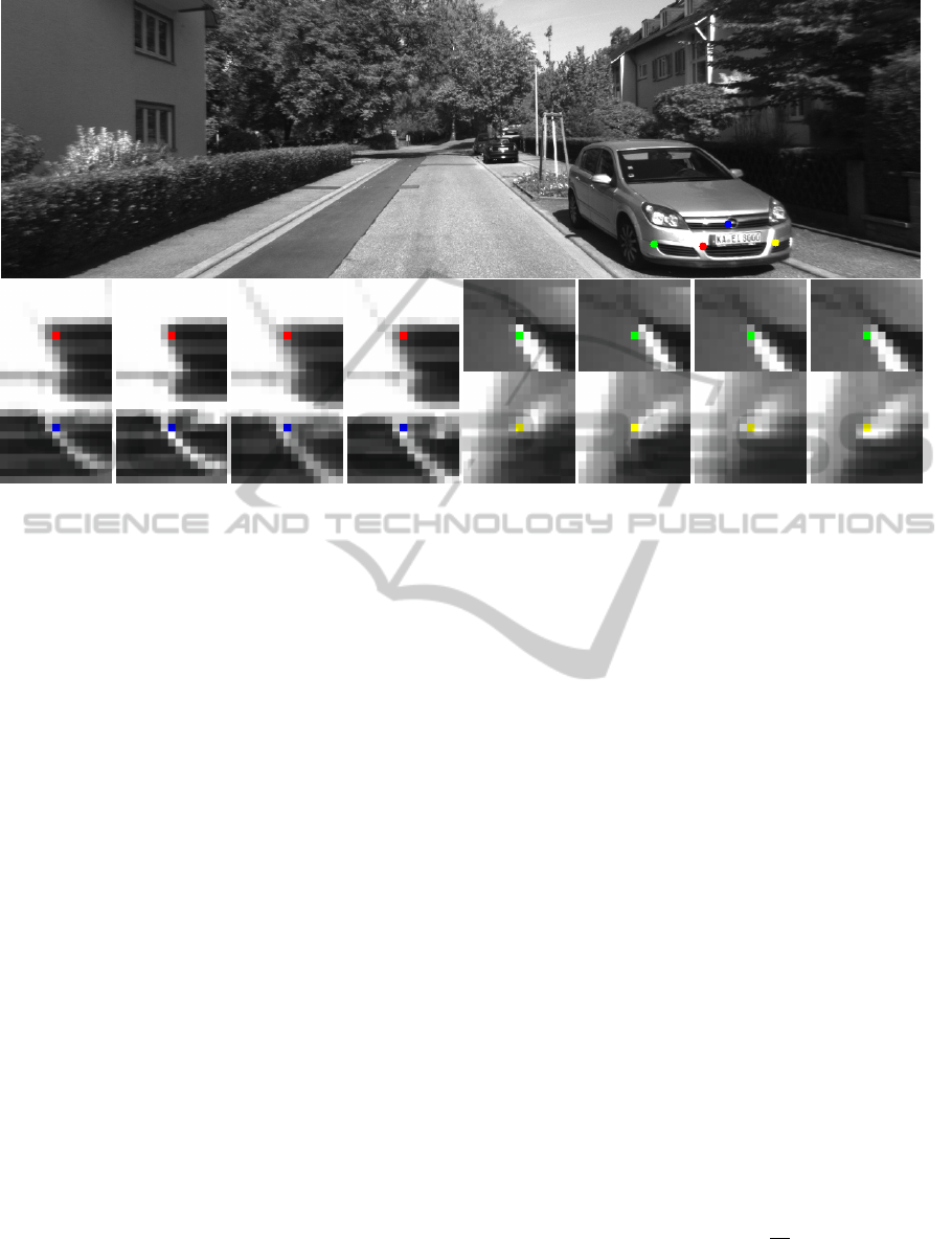
Figure 2: The image on the top corresponds to the frame #1 of the training KITTI sequence 03. Four point features have been
annotated with different colors. The four bottom images show four 15x15 patches around each feature point in four different
images (current-left, current-right, previous-left, previous-right). The localization error in the four images is less than 1 pixel.
However, the reprojection errors evaluated for groundtruth motion are around 7 pixels as shown in Table 1.
4.3 Learning the Stereoscopic
Deformation Field
We hypothesize that the disturbance in the reprojec-
tion error distribution shown in Figure 3 is caused
by inaccurate image rectification arising from the
insufficient capacity of the underlying radial dis-
tortion model. Therefore, we devise a technique
for correcting the camera calibration by exploiting
groundtruth motion. After seeing that mean values of
the vector errors deviate from zero and contain bias
following some specific patterns we decided to try
to learn the deformation field across discrete image
cells. Each element of the deformation field contains
two free parameters describing the translational shift
on u and v image axes in the corresponding image
cell. We differentiate between left and right camera
and learn a separate deformation field for each of
them. In order to define the cost function for learning
the deformation field we denote D
l
u
, D
l
v
, D
r
u
, D
r
v
as the
deformation matrices for u and v axes and left and
right cameras respectively. The motion parameters
R
t
and t
t
in each frame t are taken from groundtruth
data. Now if we define d
d
d() to be a simple function
which takes an image point, determines to which cell
of the image it belongs and uses a corresponding
values from deformation matrices to apply the defor-
mation, we can formulate the following optimization:
argmin
D
l
u
,D
l
v
,D
r
u
,D
r
v
M
∑
t=1
N
∑
i=1
{l,r}
∑
k
k
˜
q
k
i,t
− π(X
i,t−1
, R
t
, t
t,k
)k
2
(6)
˜
q = d
d
d(q, D
u
, D
v
)
In order to optimize the deformation field loss
function, we collect the inlier tracks in all sequences
by filtering them with groundtruth motion using a
fixed error threshold. The collected tracks are seri-
alized, saved to disk and later used by the optimiza-
tion method which learns the stereoscopic deforma-
tion field. We minimize the cost function (6) using
the Levenberg-Marquardt method which, in our ex-
periments, converged faster than the line-search gra-
dient descent methods to the same minimum. Note
that the set of point features typically contains many
outliers, since we only filter them with a permissive
threshold on the reprojection error with respect to the
groundtruth motion. This threshold has to be large
enough in order to capture the impact of larger re-
projection errors as we move further from the image
center (cf. Figure 3). These outliers can exert a sig-
nificant impact to the least-squares optimization. To
take them into account we wrap the square loss into
the robust Cauchy loss function given with the equa-
tion (7).
ρ(s) = a
2
log(1 +
s
a
2
) (7)
Here the square loss output is denoted with s. By
using the parameter a one can change the scale at
ImprovingtheEgomotionEstimationbyCorrectingtheCalibrationBias
351

(a) Distribution of reprojection error vector norms in the left camera. Darker colors correspond to the lower values. The error
increases in all directions from the minimum which is close to the image center.
16200 43960 60983 88632 159975 219012 167876 144061 171021 150130 100560 62776 39794 22913 8473
24992 79327 109810 141739 204386 315533 406393 384943 292353 216475 139156 98441 73760 45355 17461
27681 85761 122120 155581 216661 317709 424874 429657 290620 202883 141765 108101 86203 57941 22437
10618 46860 81195 115466 154868 174008 156019 131885 184310 155856 112752 80602 62472 44032 16037
1232 9360 18940 27301 38172 42210 38151 35922 40402 46551 41481 31306 26138 16588 5785
(b) Number of observed points in each cell.
0.35 0.367 0.374 0.344 0.301 0.277 0.267 0.272 0.262 0.267 0.292 0.295 0.314 0.334 0.332
0.383 0.369 0.367 0.337 0.293 0.27 0.249 0.245 0.254 0.267 0.292 0.308 0.334 0.367 0.36
0.359 0.369 0.36 0.333 0.297 0.274 0.254 0.249 0.263 0.283 0.305 0.326 0.349 0.373 0.35
0.417 0.439 0.436 0.411 0.386 0.363 0.342 0.343 0.333 0.352 0.381 0.395 0.398 0.398 0.394
0.606 0.587 0.581 0.573 0.538 0.508 0.477 0.474 0.465 0.455 0.462 0.483 0.492 0.494 0.518
(c) Reprojection error L2-norm means.
-0.129 -0.144 -0.171 -0.159 -0.118 -0.0729 -0.0487 -0.0328 -0.0125 -0.0196 -0.0245 -0.0176 -0.0328 -0.0658 -0.0713
-0.141 -0.124 -0.153 -0.132 -0.0902 -0.0489 -0.0238 -0.022 -0.0277 -0.0394 -0.053 -0.0626 -0.0824 -0.112 -0.125
-0.112 -0.116 -0.138 -0.115 -0.0814 -0.0509 -0.031 -0.0291 -0.0455 -0.0638 -0.0922 -0.0887 -0.109 -0.152 -0.144
-0.182 -0.188 -0.188 -0.168 -0.152 -0.0982 -0.0741 -0.0574 -0.0696 -0.0849 -0.115 -0.121 -0.116 -0.146 -0.134
-0.304 -0.255 -0.243 -0.234 -0.191 -0.131 -0.0874 -0.0892 -0.0945 -0.105 -0.108 -0.122 -0.116 -0.148 -0.18
(d) Reprojection error means on the u axis.
0.0173 0.0252 0.0219 0.0049 -0.00545 -0.00162 0.0048 0.00391 0.00424 0.0178 0.0288 0.0401 0.0601 0.0779 0.0624
0.0169 0.0372 0.0431 0.0345 0.0197 0.0146 0.00939 0.0117 0.0173 0.0265 0.0467 0.0613 0.0726 0.0801 0.0512
0.0255 0.05 0.0545 0.0499 0.0425 0.0345 0.0234 0.0204 0.0325 0.0407 0.0517 0.0581 0.07 0.069 0.0369
0.0641 0.0826 0.0884 0.0924 0.0891 0.0773 0.0769 0.065 0.0779 0.0842 0.0821 0.0921 0.0918 0.0811 0.053
0.144 0.131 0.131 0.148 0.126 0.141 0.128 0.128 0.121 0.133 0.149 0.156 0.166 0.175 0.15
(e) Reprojection error means on the v axis.
0.25 0.238 0.216 0.168 0.117 0.106 0.109 0.119 0.103 0.117 0.155 0.167 0.192 0.209 0.226
0.333 0.267 0.213 0.174 0.131 0.116 0.0947 0.0883 0.104 0.128 0.149 0.181 0.207 0.247 0.235
0.272 0.263 0.224 0.187 0.141 0.12 0.103 0.0968 0.116 0.144 0.169 0.218 0.243 0.243 0.23
0.352 0.347 0.336 0.291 0.228 0.218 0.205 0.237 0.193 0.213 0.27 0.294 0.319 0.296 0.306
0.567 0.543 0.555 0.509 0.452 0.42 0.424 0.437 0.416 0.374 0.386 0.416 0.418 0.382 0.448
(f) Reprojection error variances on the u axis.
0.118 0.131 0.138 0.125 0.123 0.131 0.128 0.13 0.136 0.126 0.135 0.125 0.115 0.11 0.0955
0.134 0.14 0.143 0.131 0.118 0.123 0.116 0.109 0.117 0.113 0.124 0.115 0.117 0.12 0.105
0.119 0.146 0.144 0.133 0.121 0.118 0.11 0.113 0.106 0.108 0.114 0.111 0.114 0.115 0.0932
0.129 0.16 0.167 0.158 0.17 0.169 0.145 0.143 0.14 0.152 0.164 0.151 0.132 0.124 0.116
0.258 0.258 0.25 0.262 0.299 0.289 0.23 0.232 0.243 0.213 0.206 0.227 0.231 0.207 0.193
(g) Reprojection error variances on the v axis.
Figure 3: Distribution of the reprojection error evaluated in groundtruth motion for sequence number 00 in KITTI dataset.
VISAPP2015-InternationalConferenceonComputerVisionTheoryandApplications
352

Figure 4: Heat map visualization of the distribution of re-
projection error norms for the left camera image on the
Tsukuba stereo dataset.
which robustification takes place.
4.4 Integrating the Deformation Field
in Motion Estimation
We will now integrate the learned stereoscopic defor-
mation field into the expression (3) and define a new
reprojection error cost function which applies the de-
formation field to all points before the optimization
step. In order to achieve smooth deformation transi-
tions, we compute the bilinear interpolation between
the four cells of the deformation field which surround
the point x
k
i,t
. In case when the bilinear interpolation
is not possible we use linear interpolation (close to
image edges) or we do not interpolate (close to im-
age corners). Let us denote the interpolation function
with i
i
i(). Then the proposed cost function for recover-
ing the camera motion can be formulated as follows:
argmin
R,t
N
∑
i=1
{l,r}
∑
k
k
ˆ
q
k
i,t
− π(X
i,t−1
, R, t
k
)k
2
(8)
ˆ
q = i
i
i(q, D
u
, D
v
)
5 EXPERIMENTAL RESULTS
The KITTI odometry benchmark contains 11 training
sequences with available groundtruth motion. These
11 sequences have been acquired with three differ-
ent camera setups each of which has a distinct set
of calibration parameters. We focus on the training
sequences 04-10, which constitute the largest group
of video sequences acquired with the same camera
setup. Our experiments analyze the accuracy of the
recovered camera motion according to the standard
KITTI evaluation criteria (Geiger et al., 2013)
1
. We
compare the performance of the proposed approach
for correcting the calibration bias by a stereoscopic
deformation field with two variants based on the lib-
viso library
2
. All compared algorithms employ tracks
extracted by our tracker described in Subsection 3.1.
The tracker has been configured with the same set of
parameters in all experiments.
5.1 Baseline and the Feature Weighting
The two libviso based variants differ in whether the
procedure which we call feature weighting is applied
or not. The simpler of these two variants (the one
without feature weighting) shall be referred to as the
baseline. Feature weighting can also be viewed as
a way to improve the recovered camera motion by
compensating inadequate calibration. This proce-
dure weights the reprojection error residuals kq
k
i,t
−
π(X
i,t−1
, R, t
k
)k
2
and the corresponding Jacobians of
the Gauss-Newton optimization according to the hor-
izontal distance of q
k
i,t
from the image origin. The
libviso library determined these weights as follows:
w
i
=
|u
i
− c
u
|
|c
u
|
+ 0.05
−1
(9)
We did not find any explanation in the paper about
libviso for how the equation (9) was chosen.
5.2 Leave One Out Evaluation
We test the impact of the proposed approach for cor-
recting the camera calibration by a stereoscopic defor-
mation field by leave-one-out evaluation on the train-
ing sequences 04-10. Therefore, we learn the stereo-
scopic deformation field (D
l
u
, D
l
v
, D
r
u
, D
r
v
) on six se-
quences and test its performance on the remaining se-
quence. This step is repeated seven times. The ob-
tained results are presented in Tables 2 and 3. Please
note that the columns labeled trans. show the relative
translational error of the recovered motion in percents
of the traveled distance, while the columns labeled
rot. show the relative rotation error in degrees per
meter. The tables show that the proposed approach
significantly improves the accuracy of the recovered
camera motion both with respect to the baseline im-
plementation and with respect to the feature weight-
ing. in all of the seven experiments.
1
A script for evaluating the accuracy is available at:
http://kitti.is.tue.mpg.de/kitti/devkit odometry.zip.
2
The libviso library can be accessed at:
http://www.cvlibs.net/software/libviso/.
ImprovingtheEgomotionEstimationbyCorrectingtheCalibrationBias
353
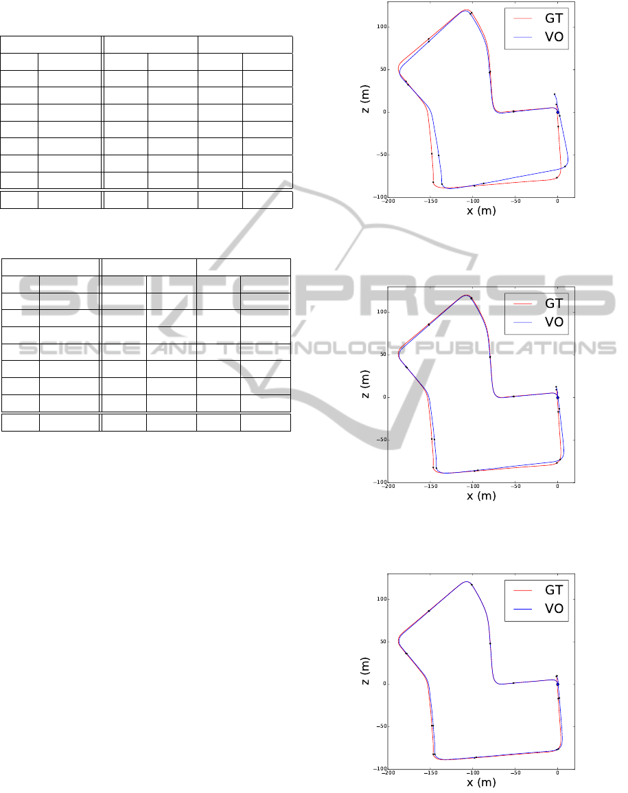
Table 2: Leave one out evaluation: baseline vs stereoscopic
deformation field (DF).
KITTI Baseline With DF
Seq. length trans. rot. trans. rot.
04 394 m 1.14 0.0094 0.78 0.0068
05 2206 m 1.29 0.0095 0.43 0.0030
06 1233 m 1.30 0.0069 0.53 0.0047
07 695 m 2.02 0.0221 0.40 0.0034
08 3223 m 1.45 0.0087 1.02 0.0048
09 1705 m 1.51 0.0067 0.97 0.0050
10 920 m 0.80 0.0067 0.70 0.0040
All 10 376 m 1.386 0.0089 0.771 0.0043
Table 3: Leave one out evaluation: baseline vs feature
weighting (FW).
KITTI Baseline With FW
Seq. length trans. rot. trans. rot.
04 394 m 1.14 0.0094 0.63 0.0027
05 2206 m 1.29 0.0095 0.70 0.0047
06 1233 m 1.30 0.0069 0.75 0.0041
07 695 m 2.02 0.0221 0.86 0.0083
08 3223 m 1.45 0.0087 1.10 0.0056
09 1705 m 1.51 0.0067 1.16 0.0041
10 920 m 0.80 0.0067 0.65 0.0042
All 10376 m 1.386 0.0089 0.933 0.0051
5.3 Case Study: The Sequence 07
According to Table 2, the translational accuracy of
the motion recovered by the baseline approach is
2.02%. Feature weighting improves that result to
0.86%. Finally, the stereoscopic deformation field
further improves the accuracy to 0.40%. The 2D plots
of the reconstructed three paths are compared to the
groundtruth motion in Figures 5, 6 and 7.
5.4 Implementation
We have implemented all the described methods and
experiments in C++. The OpenMP framework has
been used to parallelize feature tracking and motion
estimation. The implementation is based on the lib-
viso library which was modified at several places in
order to promote parallel execution and to support the
track correction with the previously calibrated stereo-
scopic deformation field.
In all experiments the resolution of the deforma-
tion field was set to 21×69 bins in each of the two
stereo images.
We implemented the optimization defined in ex-
pression (6) by using the Ceres Solver (Agarwal et al.,
2014), an open source C++ library for modeling and
Figure 5: The reconstructed camera motion along the se-
quence 07 recovered without the stereoscopic deformation
field and without the feature weighting (blue) is compared
to the groundtruth camera motion (red).
Figure 6: The reconstructed camera motion along the se-
quence 07 recovered with the feature weighting and without
the stereoscopic deformation field (blue) is compared to the
groundtruth camera motion (red).
Figure 7: The reconstructed camera motion along the se-
quence 07 recovered with the stereoscopic deformation field
and without the feature weighting (blue) is compared to the
groundtruth camera motion (red).
VISAPP2015-InternationalConferenceonComputerVisionTheoryandApplications
354

solving large nonlinear least squares problem. One
nice feature of the Ceres Solver is that it supports au-
tomatic differentiation if the cost function is written
in the appropriate form.
6 CONCLUSION
Preliminary experiments in stereoscopic egomotion
estimation had revealed that subpixel accuracy and
multi-frame optimization have a substantially larger
impact when applied to the artificial Tsukuba dataset
than in the case of the KITTI dataset. We have
decided to more closely investigate the peculiar
KITTI results by observing the reprojection error
of two-frame point-feature correspondences under
groundtruth camera motion. The performed case-
study analyses pointed out many near-to perfect cor-
respondences with large reprojection errors. Addi-
tional experiments have shown that the means and the
variances of the reprojection error significantly de-
pend on the image coordinates of the three point fea-
tures involved. In particular, we noticed that the re-
projection error bias tends to be stronger as the point
features become closer to the image borders. We have
hypothesized that this disturbance is caused by inac-
curate image calibration and rectification which could
easily arise due to insufficient capacity of the under-
lying radial distortion model.
In order to test our hypothesis, we have designed
a technique to calibrate a discrete stereoscopic de-
formation field above the two rectified image planes,
which would be able to correct deviations of a real
camera system from the radial distortion model. The
devised technique performs a robust optimization of
the reprojection error in validation videos under the
known groundtruth motion. The calibrated deforma-
tion field has been employed to correct the feature lo-
cations used to estimate the camera motion in the test
videos. We have compared the accuracy of the es-
timated motion with respect to the two baseline ap-
proaches operating on original point features. The
experimental results confirmed the capability of the
calibrated deformation field to improve the accuracy
of the recovered camera motion in independent test
videos, that is in videos which have not been seen dur-
ing the estimation of the deformation field.
In our future work we would like to evaluate dif-
ferent regularization approaches in the loss function
used to calibrate the stereoscopic deformation field.
We also wish to evaluate the impact of the estimated
correction of the calibration bias to the multi-frame
bundle adjustment optimization.
ACKNOWLEDGEMENTS
This research has been supported in part by the Eu-
ropean Union from the European Regional Develop-
ment Fund by the project IPA2007/HR/16IPO/001-
040514 ”VISTA - Computer Vision Innovations for
Safe Traffic”.
This work has been supported in part by Croatian
Science Foundation under the project I-2433-2014.
REFERENCES
Agarwal, S., Mierle, K., and Others (2014). Ceres solver.
http://ceres-solver.org.
Badino, H. and Kanade, T. (2011). A head-wearable short-
baseline stereo system for the simultaneous estimation
of structure and motion. In IAPR Conference on Ma-
chine Vision Application, pages 185–189.
Badino, H., Yamamoto, A., and Kanade, T. (2013). Visual
odometry by multi-frame feature integration. In First
International Workshop on Computer Vision for Au-
tonomous Driving at ICCV.
Diosi, A., Segvic, S., Remazeilles, A., and Chaumette, F.
(2011). Experimental evaluation of autonomous driv-
ing based on visual memory and image-based visual
servoing. IEEE Transactions on Intelligent Trans-
portation Systems, 12(3):870–883.
Fraundorfer, F. and Scaramuzza, D. (2012). Visual odom-
etry: Part ii: Matching, robustness, optimization,
and applications. Robotics & Automation Magazine,
IEEE, 19(2):78–90.
Geiger, A., Lenz, P., Stiller, C., and Urtasun, R. (2013).
Vision meets robotics: The kitti dataset. International
Journal of Robotics Research (IJRR).
Geiger, A., Lenz, P., and Urtasun, R. (2012). Are we ready
for autonomous driving? the kitti vision benchmark
suite. In Conference on Computer Vision and Pattern
Recognition (CVPR).
Geiger, A., Ziegler, J., and Stiller, C. (2011). Stereoscan:
Dense 3d reconstruction in real-time. In IV. Karlsruhe
Institute of Technology.
Harris, C. and Stephens, M. (1988). A combined corner
and edge detector. In Proceedings of the Alvey Vision
Conference, pages 147–152.
Hartley, R. I. and Kang, S. B. (2005). Parameter-free radial
distortion correction with centre of distortion estima-
tion. In ICCV, pages 1834–1841.
Howard, A. (2008). Real-time stereo visual odometry for
autonomous ground vehicles. In IROS, pages 3946–
3952.
Konolige, K. and Agrawal, M. (2008). Frameslam:
From bundle adjustment to real-time visual mapping.
Robotics, IEEE Transactions on, 24(5):1066–1077.
Konolige, K., Agrawal, M., and Sol
`
a, J. (2007). Large-scale
visual odometry for rough terrain. In ISRR, pages
201–212.
ImprovingtheEgomotionEstimationbyCorrectingtheCalibrationBias
355

Kreso, I., Sevrovic, M., and Segvic, S. (2013). A novel geo-
referenced dataset for stereo visual odometry. CoRR,
abs/1310.0310.
Martull, S., Peris, M., and Fukui, K. (2012). Realistic cg
stereo image dataset with ground truth disparity maps.
Technical report of IEICE. PRMU, 111(430):117–
118.
Moravec, H. P. (1980). Obstacle Avoidance and Naviga-
tion in the Real World by a Seeing Robot Rover. PhD
thesis, Stanford University.
Moravec, H. P. (1981). Rover visual obstacle avoidance. In
IJCAI, pages 785–790.
Nedevschi, S., Popescu, V., Danescu, R., Marita, T., and
Oniga, F. (2013). Accurate ego-vehicle global local-
ization at intersections through alignment of visual
data with digital map. IEEE Transactions on Intel-
ligent Transportation Systems, 14(2):673–687.
Nist
´
er, D., Naroditsky, O., and Bergen, J. R. (2004). Visual
odometry. In CVPR (1), pages 652–659.
Scaramuzza, D. and Fraundorfer, F. (2011). Visual odome-
try [tutorial]. IEEE Robot. Automat. Mag., 18(4):80–
92.
Sturm, P. F., Ramalingam, S., Tardif, J., Gasparini, S., and
Barreto, J. (2011). Camera models and fundamental
concepts used in geometric computer vision. Foun-
dations and Trends in Computer Graphics and Vision,
6(1-2):1–183.
Vogel, C., Roth, S., and Schindler, K. (2014). View-
consistent 3d scene flow estimation over multiple
frames. In ECCV, pages 263–278.
Zhang, Z. (2000). A flexible new technique for camera
calibration. IEEE Trans. Pattern Anal. Mach. Intell.,
22(11):1330–1334.
VISAPP2015-InternationalConferenceonComputerVisionTheoryandApplications
356
