
Segmentation of Optic Disc and Blood Vessels in Retinal Images
using Wavelets, Mathematical Morphology and Hessian-based
Multi-scale Filtering
Luiz Carlos Rodrigues and Maur
´
ıcio Marengoni
Department of Electrical Engineering, Universidade Presbiteriana Mackenzie, S
˜
ao Paulo, Brazil
Keywords:
Retinal Images, Mathematical Morphology, Wavelets, Multi-scale Filter.
Abstract:
A digitized image captured by a fundus camera provides an effective, inexpensive and non-invasive resource
for the assessment of vascular damage caused by diabetes, arterial hypertension, hypercholesterolemia and
aging. These unhealthy conditions may have very serious consequence like hemorrhages, exudates, branch
retinal vein occlusion, leading to the partial or total loss of vision capabilities. This study has focus on the
computer vision techniques of image segmentation required for a completely automated assessment system
for the vascular conditions of the eye. The study here presented proposes a new algorithm based on wavelets
transforms and mathematical morphology for the segmentation of the optic disc and a Hessian based multi-
scale filtering to segment the vascular tree in color eye fundus photographs. The optic disc and vessel tree, are
both essential to the analysis of the retinal fundus image. The optic disc can be identified by a bright region
on the fundus image, for its segmentation we apply Haar wavelets transform to obtain the low frequencies
representation of the image and then apply mathematical morphology to enhance the segmentation. The tree
vessel segmentation is achieved using a Hessian-based multi-scale filtering that, based on its second order
derivatives, explores the tubular shape of a blood vessel to classify the pixels as part, or not, of a vessel. The
proposed method is being developed and tested based on the DRIVE database, which contains 40 color eye
fundus images.
1 INTRODUCTION
The automated retinal image analysis has became,
during the recent years, a large field of research due
the advances in computer vision techniques and im-
age acquisition. This growing interest is due to sev-
eral factors outlined below (Rossant et al., 2011):
1. Eye fundus is the only location of the human body
where the blood vessels can be visualized non in-
vasively in vivo.
2. Retinal images can be produced, distributed and
processed in a relatively inexpensive way.
3. Retinal vessels and arteries are strong an trustable
indicators of pathologies as diabetes, arterial hy-
pertension and high level of cholesterol.
Beyond the context of the clinical research, automated
methods of retinal images analysis have a social high
importance since they create the possibility to real-
ize very quickly exams in a large number of images,
saving time and human resources and still offering
more quantitative metrics than the human observation
techniques. The proposed method was developed and
tested on the DRIVE (Digital Retinal Images for Ves-
sel Extraction) database, which contains 40 color eye
fundus images.Each image is captured using 8 bits
per color plane and has the size of 593 x 576 pix-
els. The FOV of each image is circular with a diam-
eter of approximately 540 pixels. For research ref-
erence, manual segmentations are also available and
have been performed by three independent observers.
The database is decomposed in a training set of 20
images and a test set of 20 images (Staal et al., 2004).
1.1 Related Works
Many researches have been developed and were re-
lated by (Fraz et al., 2012) . Algorithms and method-
ologies for detecting retinal blood vessels can be
grouped into techniques based on pattern recogni-
tion,wavelets, morphological processing,matching fil-
tering, vessel tracking, and model-based algorithms.
The pattern recognition algorithm can be subdivided
in two branches: supervised methods and unsuper-
617
Rodrigues L. and Marengoni M..
Segmentation of Optic Disc and Blood Vessels in Retinal Images using Wavelets, Mathematical Morphology and Hessian-based Multi-scale Filtering.
DOI: 10.5220/0005317006170622
In Proceedings of the 10th International Conference on Computer Vision Theory and Applications (VISAPP-2015), pages 617-622
ISBN: 978-989-758-089-5
Copyright
c
2015 SCITEPRESS (Science and Technology Publications, Lda.)
vised methods. Supervised methods utilizes ground
truth data for the classification of vessels based on
a given vector of characteristics. These methods in-
clude neural network(Mar
´
ın et al., 2010), principal
component analysis (Sinthanayothin et al., 1999), k-
nearest neighbor classifier and ridge based primitives
classification (Staal et al., 2004), support vector ma-
chine(SVM) classification (Ricci and Perfetti, 2007)
and feature-based Adaboost classifier (Lupas et al.,
2010). The unsupervised methods work without hav-
ing any prior labeling knowledge, and do not have
a previous training phase. Some reported methods
are fuzzy C-means clustering algorithm. radius-based
clustering algorithm, maximum likelihood estimation
of vessel parameters, matched filtering along with
specially weighted fuzzy C-means clustering (Kande
et al., 2010).
2 THEORETICAL BACKGROUND
2.1 Wavelets Transform (WT)
The wavelet transform is a signal decomposition as a
combined basis functions set, obtained by dilation(a)
and translations (b) of a single prototype wavelet ψ(t).
Thus, the WT of a signal x(t) is defined as
W (a, b) =
Z
+∞
−∞
f (t)
1
p
|a|
ψ
∗
t −b
a
dt (1)
The greater the scale factor a is, the wider is the
basis function and consequently, the corresponding
coefficients gives information about lower frequency
components of the signal, and vice versa. In this way,
the temporal resolution is higher at high frequencies,
achieving the property that the analysis window com-
prises the same number of periods for any central fre-
quency. If the prototype wavelet ψ(t) is the derivative
of a smoothing function θ(t), it can be shown (Burrus
et al., 1998) that the wavelet transform of a signal x(t)
at scale a is:
W (a, b) =
Z
+∞
−∞
f (t)
1
p
|a|
ψ
∗
t −b
a
dt (2)
where θ(t) = (
1
√
a
θ
t
a
) is the scaled version of the
smoothing function. The wavelet transform at scale a
is proportional to the derivative of the signal filtered
version with a smoothing impulse response at scale a.
Therefore the zero crossing of the WT corresponds to
the local maxima or minima of the smoothed signal
at different scales and the maximum absolute values
of the wavelet transforms are associated with maxi-
mum slopes in the filtered signal. In this study we
are interested in images processing which are com-
posed of slopes and local maxima (or minima) at dif-
ferent scales occurring at different level of intensity
of the pixels. The scale factor a or the translation pa-
rameter b can be discretized. The usual choice is to
follow a dyadic grid on the time-scale plane: a = 2
k
and b = 2
k
l. This transform is called dyadic wavelet
transform with basis functions (Addison, 2005)
ψ
k,l
(t) = 2
(−
k
2
)
ψ(2
k
t −l) where k, l ∈ Z
+
(3)
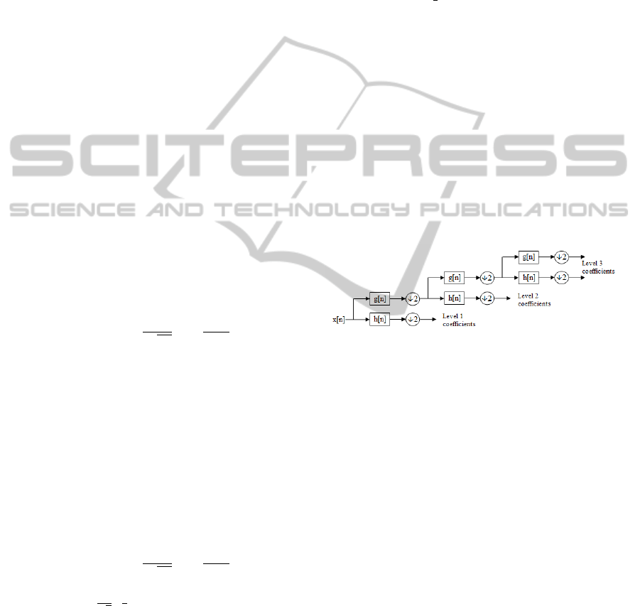
For discrete-time signals, the dyadic discrete
wavelet transform(DWT) is equivalent , according to
Mallat’s algorithm (Mallat, 1989), to an octave filter
bank and can be implemented as a cascade of identical
cells, low-pass and high-pass finite impulse response
[FIR] filters, as illustrated in Fig. 1. From the trans-
formed coefficients W
2
k
x[2
k
l] and the low-pass resid-
ual, the original sign can be rebuilt using a reconstruc-
tion filter bank. The down samplers after each filter in
Fig.1 remove the redundancy of the signal represen-
tation. As side effects, they make the signal represen-
tation time variant and reduce the temporal resolution
of the wavelet coefficient for increasing scales.
Figure 1: Mallat’s algorithm for the two filter bank imple-
mentation of DWT.
2.2 Mathematical Morphology
The word morphology refers to form and structure; in
computer vision it can be used to refer to the shape of
a region. The operations of mathematical morphology
were originally defined as set operations and shown
to be useful for processing sets of 2D points (Shapiro
and Stockman, 2001). The language of mathemati-
cal morphology is the set theory. Sets in mathemat-
ical morphology represent the shapes which are rep-
resented in binary or gray tone. The set of all black
pixels in a black white image, a binary image consti-
tutes a complete description of the binary image (Har-
alick and Sternberg, 1987). The operations of binary
morphology input a binary image B and a structuring
element S, usually another smaller binary image. The
structuring element represents a shape; it can have an
arbitrary size.
VISAPP2015-InternationalConferenceonComputerVisionTheoryandApplications
618

2.3 Scale-Space and Hessian-based
Filtering
The scale-space theory is a framework conceived for
the representation of an image, or signal, in mul-
tiple scales, or apertures (Witkin, 1983). Its moti-
vation comes from the resemblance of close recep-
tive field profiles of human visual system and in-
tents the representation of an object in multiple scales
simultaneously, obeying some axioms like linearity,
spacial shift invariance, isotropy and scale invari-
ance (Florack et al., 1992). Based on scale-spaces
theory (Koenderink, 1984), Frangi et al. (Frangi et al.,
1998) developed a multi scale approach to the use of
the eigenvalues of the Hessian to determine locally
the likelihood that a pixel may be considered a part
of a vessel. This conceives the vessel enhancement as
a filtering process that searches for geometrical struc-
tures which may be considered a tubular shape. The
idea is, given a point x
0
in an image, to consider the
Taylor expansion in its neighbourhood,
L(x
0
+ δx
0
, s) ≈ L(x
0
+ x
0
, s) + δx
T
0
∆
0,s
+ δx
T
0
H
0,s
δx
0
(4)
Where ∆
0,s
is the gradient vector and H represents the
Hessian matrix, a 2-by-2 matrix containing the sec-
ond partial derivatives of a function, as shown for a
2D image I(x, y) in (5) The Hessian matrix contains
also all the second order information needed for each
pixel. To extract information about contrast and direc-
tion of a pixel from the Hessian matrix its eigenvalues
are calculated.
H(x, y) =
∂
2
I
∂x
2
∂
2
I
∂x∂y
∂
2
I
∂x∂y
∂
2
I
∂x
2
(5)
Like the image I, the Hessian is also a discrete
function and may be approximated to a continuous
function using the 2-dimensional Gaussian (6) filter
and the convolution differentiation property accord-
ing (7)
G(x, y) = e
−
1
2
(
x
2
σ
2
1
+
y
2
σ
2
2
)
(6)
H(x, y) ≈G∗
∂
2
I
∂x
2
∂
2
I
∂x∂y
∂
2
I
∂x∂y
∂
2
I
∂x
2
=
∂
2
G
∂x
2
∂
2
G
∂x∂y
∂
2
G
∂x∂y
∂
2
G
∂x
2
∗I(x, y),
(7)
where ∗ is the convolution symbol. Let |λ
1
| ≤ |λ
2
|
represent the two eigenvalues calculated from the
Hessian matrix and u
1
and u
2
the correspondent
eigenvectors. Since |λ
1
| is the eigenvalue of small-
est magnitude it corresponds to the eigenvector, u
1
,
pointing out the direction of smallest curvature, and
|λ
2
| corresponds to the eigenvector u
2
pointing out
the direction of largest curvature. In terms of a blood
vessel, it means that u
1
is parallel to longitudinal axis
of the blood vessel, and |λ
1
|
∼
=
0 while u
2
is parallel to
the radial axis. With these values, two measures were
created to assess the anisotropy and the contrast of the
pixel. These measures are obtained by (8) and (9).
R
a
=
|λ
1
|
|λ
2
|
(8)
R
b
=
q
|λ
1
|
2
+ |λ
2
|
2
(9)
During the process of classification of a given
pixel, the lower R
a
higher is the probability of the
pixel be part of a vessel.
R
b
will be low if both eigenvalues are small for the
lack of contrast so that larger R
b
higher is the proba-
bility of the pixel be part of a vessel.
For images where the vessels are darker than their
background, what means that these vessels are repre-
sented like valleys, the curvature will be negative so
|λ
2
| < 0.
These conclusions leaded the development of
a likelihood function, also known as ”vesselness
equation”(10) at each scale s,
V
0
(s) =
(
0 if λ
2
> 0
e
−
R
2
a
2α
2
(1 −e
−
R
2
b
2β
2
) otherwise
(10)
where α and β are thresholds which control the
sensitiviy of the line filter to the measures R
a
and R
b
.
The table 1 illustrates the possible patterns as-
sumed by the combination of the ordered eigenvalues
( |λ
1
| < |λ
2
|) for a 2D image.
Table 1: Possible patterns in 2D depending on the value of
the eigenvalues λ
k
. +/- indicate the sign of the eigenvalues.
Eigenvalues
λ
1
λ
2
Orientation Pattern
Noisy Noisy noisy, no preferred direction
Low High- tubular structure (bright)
Low High+ tubular structure (dark)
High- High- blob-like structure (bright)
High+ High+ blob-like structure (dark)
3 METHODS
3.1 Optic Disc Segmentation
In this section we describe the process to extract the
localization of the optic disc analyzing the eye fundus
SegmentationofOpticDiscandBloodVesselsinRetinalImagesusingWavelets,MathematicalMorphologyand
Hessian-basedMulti-scaleFiltering
619
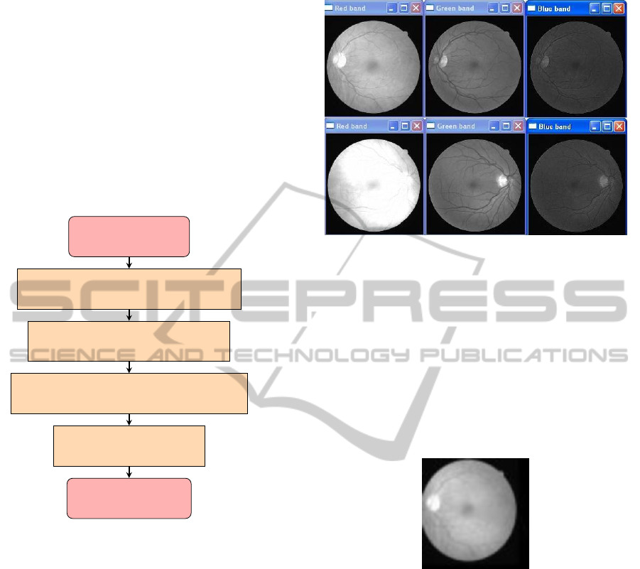
image provided by DRIVE database. The optic disc
is the region of entrance of the blood vessels and the
optic nerve into the retina. The appearance of the op-
tic disc in a color fundus image is a bright yellowish
or white region. Its contour is more or less circular
and it is interrupted by the outgoing vessels. Non rare
it may have an elliptical form due the considerable
angle between the image plane and the object plane.
The diameter may assume different sizes depending
on the patient and is in the range of 40 to 60 pixels
in 640 x 480 color images. The complete algorithm
is represented by the diagram shown in the flowchar
below.
Eye Fundus Image
Histogram analysis for band selection
Wavelet 5th Level Decomposition
Polygonal approximation to find Circles
Eliminate False Positives
Optic Disc Detected
We first read an JPG image of DRIVE image and
execute an Histogram Analysis, comparing with three
reference images that will indicate the best color band
to consider for processing. Each of our three image
reference is associated to the selection of one of the
three color bands. Higher the level of histogram simi-
larity of the input image with one of image reference,
the image reference will indicate the best band to be
processed, discarding the others two. These three im-
age reference were selected based in empirical test-
ings. The reason for this procedure is that not always
a selected color band is good enough for processing
the all set of samples, since each sample may presents
very different distribution of gray scales, increasing
the error of the algorithm. As shown in Fig. 2 for the
first test record, the upper picture, the more suitable
band to locate the optic disc in Red band, due the good
contrast. However, for second test record, shown be-
low, the best option would be the green band, once
the Red band has a very low contrast, increasing the
difficulties to locate the optic disc. Once selected, the
best band is submitted to an pyramidal Haar wavelet
Figure 2: Above the RGB bands of the first record of set
test set. Below the RGB bands of the second record of the
test set.
decomposition that produce a sub bands vector, con-
taining the frequencies approximations of the image.
The 5th level of decomposition with 37x36 pixels is
then resized and interpolated to an original size of the
image, 592 x 576. We then convert the interpolated
5th level wavelets approximation into a binary image,
applying a threshold of minimum pixel value of 220
and a maximum pixel value of 225. The result is show
in Fig. 3
Figure 3: Example of the 5th level of wavelet transform
signal decomposition.
3.2 Retinal Vessel Segmentation
The multi-scale vessel detection was performed for
scales between t
min
and t
max
( corresponding to σ
min
to
σ
max
). For each σ ∈hσ
min
;σ
max
ithe Hessian matrices
were calculated using (7). The the eigenvalue analy-
sis was performed using the criteria described in Sec-
tion 2.3 and the results for each scale were obtained.
The final result of the multi-scale analysis pixel-wise
maximum of obtained results over all analyzed scales.
VISAPP2015-InternationalConferenceonComputerVisionTheoryandApplications
620
4 EXPERIMENTAL RESULTS
4.1 Optic Disc Segmentation
The 20 color images of the DRIVE database were
submitted to this algorithm. In 17 images, the optic
disc was correctly localized. And in 10 images the
exact contour was also found. However, due the low
contrast we found some false positives and in two im-
ages the algorithm failed and the result was not ac-
ceptable. As a initial result it maybe considered a
good outcome, since the bad results are consequence
of abnormal optic disk that require an additional pre-
processing on the image. This pre-processing is un-
der elaboration and we intend to implement it and im-
prove significatively the process.
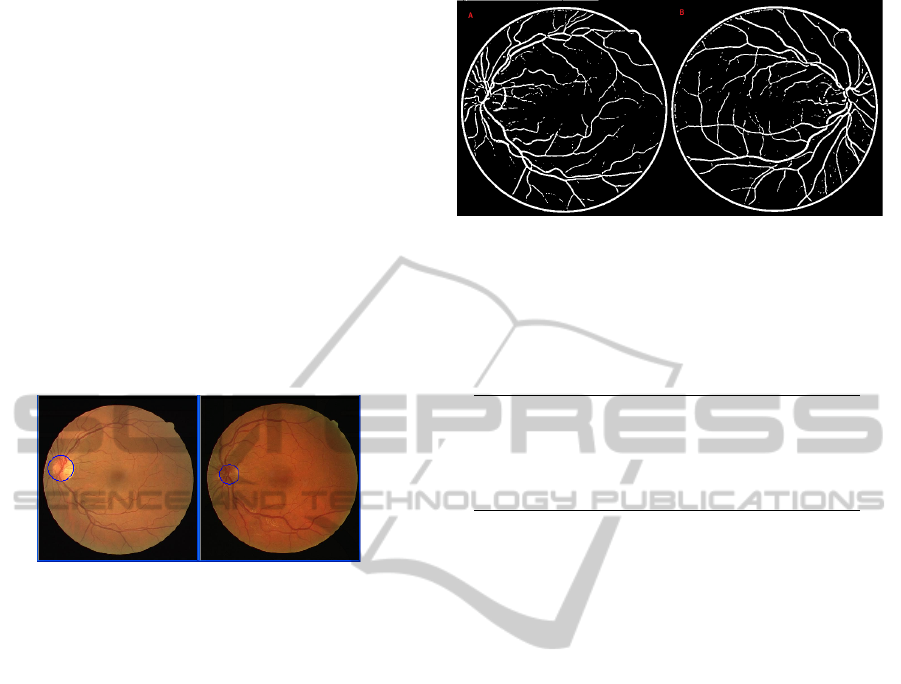
Figure 4: Two examples of optic disc outlines determined
by this method.
4.2 Retinal Vessel Segmentation
The green channel of the RGB-colored retinal image
was selected for the image processing because it nor-
mally presents a better contrast between the blood
vessels and the retinal background. DRIVE database
image makes available a binary mask for the FOV for
each record. The 20 images of DRIVE database were
used to assess this algorithm. We use these masks as
reference to determine the accuracy of our algorithm.
The first results are fully satisfactory and we obtained
good results in images with high and low contrast.
Smaller vessels that are not connected to the vascular
tree might be missed without prejudice to the purpose
of this study.
Fig. 6 shows an example of a blood vessel seg-
mentation of a green channel. The two examples are
a result of a empirical test, when we processed the
image until the sixth scale, starting with σ = 0.5, with
increments of 0.3 and R
a
= 2 and R
b
= 10.
Several studies have been made on blood vessel
segmentation using the DRIVE database. Some of
these studies are shown in the table 2:
Comparing with the other studies, it is remarkable
the average accuracy achieved by the implementation
of Hessian-based multi-scale filter without any pre-
Figure 5: This picture shows the result of the execution of
the algorithm on two DRIVE records.A) Segmentation of
the record 01-test.tif with 0,9447 of accuracy. B) Segmen-
tation of the record 02-test.tif with 0,9347 of accuracy.
Table 2: Table shows an overview of the performance of
different methods.
Method Accuracy
Human Observer 0.9473
Staal (Staal et al., 2004) 0.9442
Niemeijer (Niemeijer et al., ) 0.9416
Zana (Zana and Klein, 2001) 0.9377
This Study (Under development) 0.9269
processing, except the conversion from color to gray
scale.
5 CONCLUSION AND
DISCUSSION
Two algorithms for automatic segmentation of eye
fundus images were demonstrated in this document.
First, we demonstrated the successful application of
wavelets on the optic disc segmentation, a fundamen-
tal process in any system of identification and clas-
sification of pathologies in retinal images. We have
shown our first results and demonstrated, through the
good accuracy of the firsts results, that the technique
maybe applied with satisfactory accuracy. There are
still problems to be solved, like the images with very
low contrast on the optic disc region or with a patho-
logically abnormal optic disc. This problem may be
addressed with the variation of the wavelets scales,
or even the selection of a new type of wavelet, and
the application of a adaptive filter. These testings are
under development to be applied soon. An exemple
of bad optic disc localization by the algorithm hap-
pened in the record 34 of the training group, that have
a pathology and could not be properly localized and
classified.
We then demonstrated the applicability of
Hessian-based multi-scale filtering on segmentation
of blood vessels, as well
We have successfully shown the applicability of
SegmentationofOpticDiscandBloodVesselsinRetinalImagesusingWavelets,MathematicalMorphologyand
Hessian-basedMulti-scaleFiltering
621
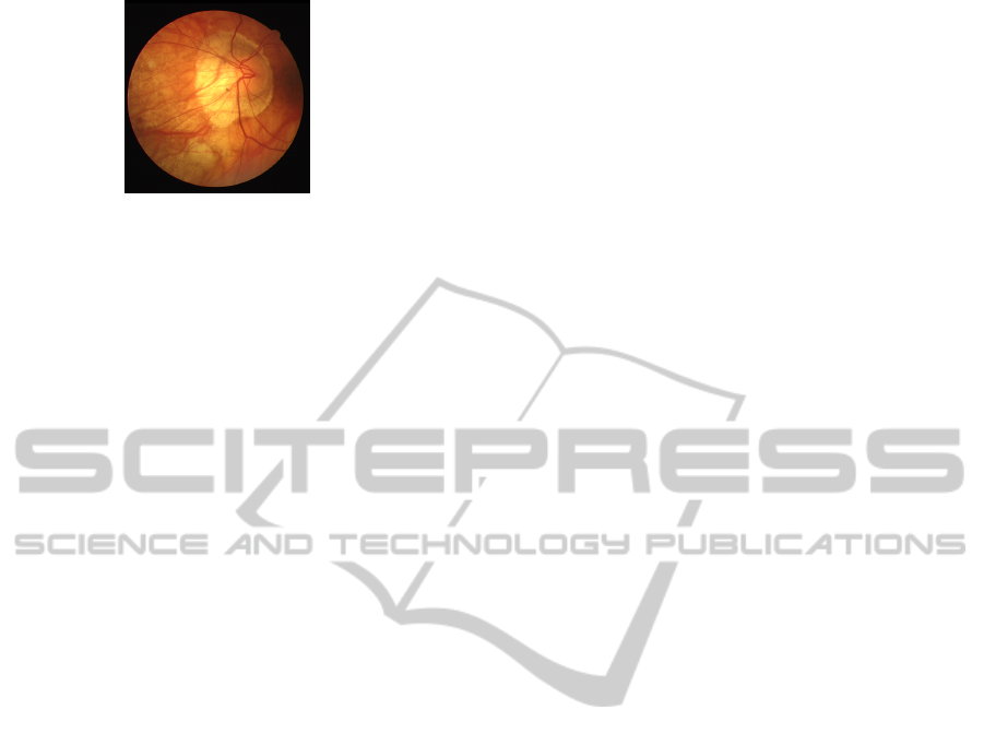
Figure 6: This picture shows an abnormal optic disc that
could not yet be properly segmented by the algorithm.
these algorithms in segmentation of retinal images
segmentation, as well the very good accuracy average
obtained, when comparing with other studies devel-
oped on the same database.
The optic disc and the vessels are fundamental for
the understanding and analysis of ocular fundus im-
ages. Our objective was to define two algorithms that
will be used as a first stage in image registration to
identify false positives in pathology detection and for
automatic classification of detected pathologies.
ACKNOWLEDGEMENTS
The authors thank Fundo Mackenzie de Pesquisa
(Mackpesquisa) from the Universidade Presbiteriana
Mackenzie for the financial support for this research.
REFERENCES
Addison, P. S. (2005). Wavelet transforms and the ECG: a
review. Physiological measurement, 26(5):R155–99.
Burrus, C. S., Gopinath, R. A., and Guo, H. (1998). In-
troduction to Wavelets and Wavelet Transforms: A
Primer.
Florack, L. M., ter Haar Romeny, B. M., Koenderink, J. J.,
and Viergever, M. a. (1992). Scale and the differen-
tial structure of images. Image and Vision Computing,
10(6):376–388.
Frangi, A. F., Niessen, W. J., Vincken, K. L., and Viergever,
M. A. (1998). Multiscale vessel enhancement filtering
1 Introduction 2 Method. 1496:130–137.
Fraz, M. M., Remagnino, P., Hoppe, a., Uyyanonvara, B.,
Rudnicka, a. R., Owen, C. G., and Barman, S. a.
(2012). Blood vessel segmentation methodologies in
retinal images–a survey. Computer methods and pro-
grams in biomedicine, 108(1):407–33.
Haralick, R. M. and Sternberg, S. R. (1987). Image Analy-
sis Morphology. (4):532–550.
Kande, G. B., Subbaiah, P. V., and Savithri, T. S. (2010).
Unsupervised Fuzzy Based Vessel Segmentation In
Pathological Digital Fundus Images. J. Med. Syst.,
34(5):849–858.
Koenderink, J. J. (1984). Biological Cybernetics The Struc-
ture of Images. 370:363–370.
Lupas, C. A., Tegolo, D., and Trucco, E. (2010). FABC
: Retinal Vessel Segmentation Using AdaBoost.
14(5):1267–1274.
Mallat, S. G. (1989). Theory for multiresolution signal de-
composition: the wavelet representation. IEEE Trans-
actions on Pattern Analysis and Machine Intelligence,
11:674–693.
Mar
´
ın, D., Aquino, A., Geg
´
undez-arias, M. E., and Bravo,
J. M. (2010). Pr E oo f Pr E oo f. pages 1–13.
Niemeijer, M., Staal, J., Ginneken, B. V., Loog, M., and
Abr, M. D. Comparative study of retinal vessel
segmentation methods on a new publicly available
database.
Ricci, E. and Perfetti, R. (2007). Retinal Blood Vessel Seg-
mentation Using Line Operators and Support Vector
Classification. Medical Imaging, IEEE Transactions
on, 26(10):1357–1365.
Rossant, F., Badellino, M., Chavillon, A., Bloch, I., and
Paques, M. (2011). A Morphological Approach for
Vessel Segmentation in Eye Fundus Images, with
Quantitative Evaluation. Journal of Medical Imaging
and Health Informatics, 1(1):42–49.
Shapiro, L. and Stockman, G. (2001). Computer Vision,
volume 2004.
Sinthanayothin, C., Boyce, J. F., Cook, H. L., and
Williamson, T. H. (1999). Automated localisation of
the optic disc, fovea, and retinal blood vessels from
digital colour fundus images. British Journal of Oph-
thalmology, 83(8):902–910.
Staal, J., Member, A., Abr
`
amoff, M. D., Niemeijer, M.,
Viergever, M. A., Ginneken, B. V., and Detection,
A. R. (2004). Ridge-Based Vessel Segmentation in
Color Images of the Retina. 23(4):501–509.
Witkin, A. P. (1983). Scale-space Filtering. In Proceedings
of the Eighth International Joint Conference on Arti-
ficial Intelligence - Volume 2, IJCAI’83, pages 1019–
1022, San Francisco, CA, USA. Morgan Kaufmann
Publishers Inc.
Zana, F. and Klein, J. C. (2001). Segmentation of vessel-
like patterns using mathematical morphology and cur-
vature evaluation. IEEE transactions on image pro-
cessing : a publication of the IEEE Signal Processing
Society, 10(7):1010–9.
VISAPP2015-InternationalConferenceonComputerVisionTheoryandApplications
622
