Automatic Road Segmentation of Traffic Images
Chiung-Yao Fang
1
, Han-Ping Chou
2
, Jung-Ming Wang
1
and Sei-Wang Chen
1
1
Dept. of Computer Science and Information Engineering, National Taiwan Normal University, Taipei City, Taiwan
2
Dept. of Information Management, Chung Hua University, Hsin-Chu City, Taiwan
Keywords: Fuzzy Decision, Shadow Set, Background-Shadow Model.
Abstract: Automatic road segmentation plays an important role in many vision-based traffic applications. It provides a
priori information for preventing the interferences of irrelevant objects, activities, and events that take place
outside road areas. The proposed road segmentation method consists of four major steps: background-
shadow model generation and updating, moving object detection and tracking, background pasting, and road
location. The full road surface is finally recovered from the preliminary one using a progressive fuzzy-
theoretic shadowed sets technique. A large number of video sequences of traffic scenes under various
conditions have been employed to demonstrate the feasibility of the proposed road segmentation method.
1
INTRODUCTION
Roads are important objects for many applications,
such as road maintenance and management (Ndoye
et al., 2011), transport planning, traffic monitoring
and measurement, traffic accident and incident
detection, car navigation, autonomous vehicles
(Perez et al., 2011), road following (Skog et al.,
2009), and driver assistance systems. Regardless of
diverse applications, road segmentation methods can
broadly be divided into two groups. One group
(Alvarez et al., 2008)(Chen et al., 2010)(Chung et
al., 2004)(Ha et al., 2009)(Ndoye et al., 2011) is
concerned with road localization in the images of
static traffic scenes, and another group (Alvarez et
al., 2011)(Courbon et al., 2009)(Obradovic et al.,
2008)(Perez et al., 2011)(Skog et al., 2009) is
devoted to the road detection in the images of
dynamic traffic scenes. The images of static scenes
are provided by stationary cameras, whereas those of
dynamic scenes are captured by movable cameras,
e.g., the cameras mounted on moving vehicles or
robots. The roads exhibiting in the images of
dynamic scenes are typically narrow-ranged, right in
front of the carriers, and close to the cameras.
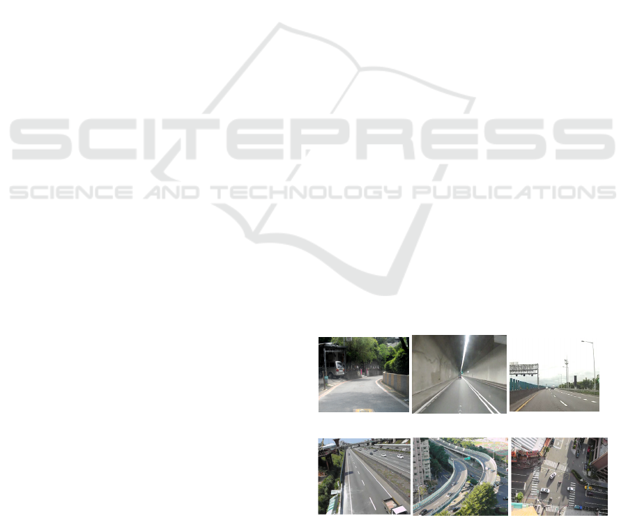
Figure 1(a) shows some examples of such images.
However, the roads presenting in the images of static
scenes can be rather different in both shape and size
due to large variations in elevation and viewing
direction from camera to camera. Figure 1(b) shows
some images of static traffic scenes. The road
detection techniques developed for the images of
static and dynamic scenes can be considerably
different. In this study, we focus on the images of
static traffic scenes, which are commonly considered
in such applications as restricted lane monitoring,
wide-area traffic surveillance, traffic parameter
measurement, traffic accident/incident detection, and
traffic law enforcement.
(a)
(b)
Figure 1: Example images of (a) dynamic traffic scenes
and (b) static traffic scenes.
Road segmentation has often been modeled as a
classification problem, in which image pixels are
categorized as either road or non-road points based
on their properties. The properties utilized have been
ranging from the low-level ones (e.g., intensity,
color, and depth) (Danescu et al., 1994)(Santos et al.,
2013)(Tan et al., 2006)(Sha et al., 2007), the mid-
level ones (e.g., texture, edge, corner, and surface
469
Fang C., Chou H., Wang J. and Chen S..
Automatic Road Segmentation of Traffic Images.
DOI: 10.5220/0005321904690477
In Proceedings of the 10th International Conference on Computer Vision Theory and Applications (VISAPP-2015), pages 469-477
ISBN: 978-989-758-090-1
Copyright
c
2015 SCITEPRESS (Science and Technology Publications, Lda.)
patch) (Santos et al., 2013)(Soquet et al., 2007), to
the high-level ones (e.g., lane markings (Wang et al.,
2004), road boundaries, and road vanishing point)
(Alvarez et al., 2008). Various techniques
characterized by different levels of pixel properties
have been developed.
There have been a large number of different
techniques proposed, such as deformable templates
(Ma et al., 2000), watershed transformation
(Beucher et al., 1994), morphological operations
(Bilodeau et al., 1992), V-disparity algorithm
(Soquet et al., 2007), probabilistic models (Danescu
et al., 1994), boosting (Santos et al., 2013)(Fritsch et
al., 2014), and neural networks (Mackeown et al.,
1994). However, currently available road
segmentation methods either dealt with the images
of dynamic traffic scenes for such applications as car
navigation, autonomous vehicles and driver
assistance systems or considered the images of static
traffic scenes of particular road types captured by
cameras with specific elevations and viewing
directions. In this paper, we present a general road
segmentation technique applicable to the traffic
images containing roads of various types, shapes and
sizes under diverse weather (e.g., clear, cloudy, and
rain days), illumination (e.g., sunlight and shadow),
and environmental (e.g., traffic jams and cluttered
backgrounds) conditions.
The proposed method consists of four major steps:
background-shadow model generation and updating,
moving object detection and tracking, background
pasting, and road localization. In terms of these four
steps, our contributions are addressed below. First,
we model the road segmentation problem as a
classification problem. The performance of
classification heavily relies on the quality of the
given road characteristics. In the background pasting
step, a method of calculating road characteristics
from reliably located road surfaces is presented.
Second, it is inevitable that uncertainties originating
from noise, errors, imprecision, and vagueness are
involved throughout the entire process. We
employed shadowed sets, which are extended from
fuzzy sets that have been well known to be an
elegant tool for coping with vague notions, to
resolve uncertainties in the final step of road
localization.
The rest of this paper is organized as follows.
Section 2 addresses the overall idea of the proposed
road segmentation method. Section 3 details the
main steps of the proposed method. Experimental
results are then demonstrated in Section 4.
Conclusions and future work are finally given in
Section 5.
2
AUTOMATIC ROAD
SEGMENTATION
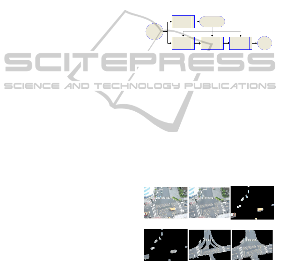
Figure 2 shows a block diagram for the proposed
road segmentation method, in which four major
steps are involved: (1) background-shadow model
generation and updating, (2) moving object detection
and tracking, (3) background pasting, and (4) road
location. The details of these four steps are discussed
in the next section. In this section, the basic idea and
novelty of the proposed method is addressed.
Input
video
sequence
Background -
shadow model
generation &
updating
Moving obj ect
detection &
tracking
Background
pasting
Road
location
Gaussian mixture
of background-
shadow model
Road are as
Figure 2: Block diagram for automatic road segmentation.
Let us look at an example shown in Figure 3 for
illustrating the proposed method. Giving a video
sequence of a traffic scene (Figure 3(a)), our
ultimate goal is to locate the road areas of the scene
(Figure 3(f)) in the video sequence. First of all, a
background-shadow model of the scene is created
from the input video sequence. This model contains
both the background and shadow information of the
scene in one model. Figure 3(b) shows a background
image of the scene provided by the model. The
model is then updated as time goes. This completes
the step of background-shadow model generation
and updating. Thereafter, moving objects are
detected and tracked over the video sequence. Figure
3(c) shows the detected objects at a certain instant in
time. Note that most of uninteresting moving
(a) (b) (c)
(d) (e) (f)
Figure 3: An example for illustrating the road
segmentation process: (a) the traffic scene under
consideration, (b) a background image of the scene, (c) the
moving objects detected at a certain time instant, (d) the
background patches corresponding to the detected moving
objects, (e) a preliminary road segment, and (f) the
recovered full road surface of the scene.
VISAPP2015-InternationalConferenceonComputerVisionTheoryandApplications
470

objects, such as flipping leaves and grasses, waving
flags, flashing lights, and the shadows
accompanying moving objects can be ignored
because they have been regarded as background
objects during building the background-shadow
model. Ideally, only moving vehicles are located in
the step of moving object detection and tracking.
However, this is usually not the case. The
subsequent steps will compensate for to some extent
this drawback.
Moving vehicles are assumed to run on the road
surface. Accordingly, the patches in the background
image, called the background patches, that
correspond to the moving objects are then extracted
and pasted on a map, called the road map, shown in
Figure 3(d). Repeating the steps of moving vehicle
detection and background pasting, a preliminary
road segment will eventually be established in the
road map depicted in Figure 3(e). This preliminary
road segment is inevitably error prone because of
imperfect moving vehicle detection. We hence
associate each pixel of the preliminary road segment
with a degree of importance that is proportional to
the times of applying background pasting to the
pixel. Statistically, noisy pixels are random in nature
and will have small degrees of importance. In the
final step of road location, the preliminary road
segment with its degrees of importance of pixels
then serves as a seed, from which the full road
region of the scene is progressively recovered by
iteratively adding background pixels to the
preliminary road segment based on both the
proximities and affinities of the pixels to the
preliminary road segment. Figure 3(f) shows the
recovered road surface of the scene.
3
IMPLEMENTATIONS OF
MAJOR STEPS
In this section, the four major steps: (1) background-
shadow model generation and updating, (2) moving
object detection and tracking, (3) background
pasting, and (4) road location, involved in the
proposed road segmentation method are detailed.
3.1
Background-shadow Model
Generation and Updating
A
In the step of background-shadow model
generation and updating, a Gaussian mixture
background-shadow (GMBS) model (Wang et al.,
2011) of the traffic scene is created, which integrates
both the background and shadow information of the
scene in one model. The reason we generate such a
model is twofold. First, shadows often confuse our
vehicle detection in view that they distort vehicle
shapes and may connect multiple vehicles into one.
Second, shadow detection is a complex and time-
consuming process. Instead of applying shadow
detection to every video image, we preserve in
advance shadow information in the GMBS model so
that we can rapidly identify shadows in images
simply relying on the shadow information provided
by the GMBS model.
3.2
Moving Object Detection and
Tracking
An approach combining the temporal differencing
and the level set techniques is employed to detect
moving objects in video sequences (Wang et al.,
2008). Temporal differencing locates the image
areas that have significant changes in characteristic
between successive images. Since the time interval
between two successive video images is extremely
short, it is reasonable to assume that the two images
have been taken under the same illumination
condition.
The level set technique (Paragios, 2006) provides
a robust method to locate objects based on their
edges even though involving imperfections. To use
this technique, the initial contours of objects have to
be provided. We group edges according to their
closeness in both distance and property (i.e., edge
magnitude) into clusters. Recall that an object may
be contained in a single component or in a number
of adjacent components in component image C
t
. The
level set method then progressively moves the
contour toward the edges inside the contour with a
speed function in a direction normal to itself. The
contour will eventually enclose the object when it
firmly hits the edges of the object.
The above moving object detection procedure is
somehow time consuming primarily due to the level
set process that is iterative in nature. We introduce
an object tracking process realized by the mean shift
technique (Comaniciu et al., 2003) to reduce the
number of object detections. Once a moving object
is detected, its subsequent locations are predicted by
the object tracking process. For each prediction, the
object detection process confirms it within the
vicinity of the predicted location. Such a cooperation
of location prediction and confirmation has
significantly expedited the moving object detection
and tracking step.
AutomaticRoadSegmentationofTrafficImages
471

3.3
Background Pasting
In the background pasting step, the background
patches corresponding to detected moving objects
are pasted on an image, called the road map.
Initially, road regions grow rapidly in the road
image. The growth will gradually slow down until
no obvious change is observed. A preliminary road
segment can be attained. In general, the preliminary
road segment contains several regions with different
characteristics, e.g., asphalt pavements, lane marks,
repaired road patches, and shadows falling on road
surfaces.
We group the image pixels of the preliminary
road segment into clusters, each of which contains
pixels having similar characteristics, using the fuzzy
c-means technique (Chen et al., 1997). Small
clusters are first ignored because they may result
from noises. Recall that each pixel of the
preliminary road segment possesses a degree of
importance that is proportional to the number of
moving vehicles passing through the pixel. We then
compute the degrees of importance for the clusters
based on those associated with their constituting
pixels. We remove the clusters with small degrees of
importance. These clusters may result from the
perspective projections of large vehicles outside of
the road region. Thereafter, for each remaining
cluster its mean of characteristics of image pixels is
calculated. Let {m
1
, m
2
, …, m
c
} be the means of
clusters, in which c is the number of clusters.
Finally, we compute the chamfer distances D of
image pixels from the preliminary road segment.
Figure 4 shows an example of the above processing.
Figure 4: Five major clusters of homogeneous regions
included in the preliminary road segment of Video 1. The
top left is the background image and the others are
homogeneous regions.
3.4
Road Location
In the road location step, the full road region is
progressively recovered from the preliminary road
segment. Figure 5 gives the algorithm of road
location. In each iteration, the degree μ(
x
) of any
image pixel
x
belonging to a road surface is first
estimated based on both its characteristic
a
(
x
) and
chamfer distance D(
x
), i.e.,
μ
(x) = wg
1
(min
1≤k≤c
{a(x)− m
k
}) + (1− w)g
2
(D(x))
, (4)
where
m
k
is the mean vector of cluster k, g
i
(·)(I = 1,
2) are Gaussian functions, and w is a weighting
factor for balancing image characteristic and
chamfer distance. The above equation states that the
more comparable the characteristic of the pixel to
that of any cluster and that the closer the pixel to the
preliminary road segment the larger the degree of
the pixel belonging to a road surface. The
characteristics
a
(
x
) and
m
k
are color vectors in our
experiments.
Having determined the membership grades of
pixels belonging to road surfaces, instead of simply
selecting a constant threshold for the membership
grades, we introduce the fuzzy theoretic shadowed
set approach (Pedrycz, 2009) to automatically
determine a threshold for separating image pixels
into road and non-road pixels. Unlike fuzzy sets that
describe vague concepts in terms of precise
membership functions (F:
X
→[,1]), shadowed sets
model vagueness with non-numeric models
(S:
X
→{0, [, 1], 1}. Function S
possesses limited
three-valued characterization and separates the
universal set
X
into three subsets S
0
, S
1
, and S
[,1]
. In
other words, shadowed sets capture the essence of
fuzzy sets at the same time reducing the numeric
burden.
Algorithm: Road Location
Input: D: Chamfer distance of preliminary road
segmentation
a
(
x
): Characteristic of image pixel
x
{m
1
, m
2
, …, m
c
}: Means of characteristic of clusters
Steps:
1.
w
← 0
2.
Computing degree of pixel
x
belong to a road surface
using
12
1
() (min{() }) (1 ) ( ())
k
kc
wg w g D
μ
≤≤
=−+−xaxm x
3.
Computing threshold using
α
*
= arg min
α
μ
(x)
μ
(x)≤
α
+ (1 −
μ
(x))− cardinality{x |
α
<
μ
(x) <1−
α
}
μ
( x)≥1−
α
Selecting α
*
as the threshold of μ(
x
) to classify pixel
x
into road and non-road points.
4.
Increase
w
and repeat 2-4 until α
*
becomes
increasing.
Figure 5: Algorithm for road location.
Let α∈(0, 1/2) be an α-cut of the membership
function in Equation (4). Accordingly, three regions,
VISAPP2015-InternationalConferenceonComputerVisionTheoryandApplications
472
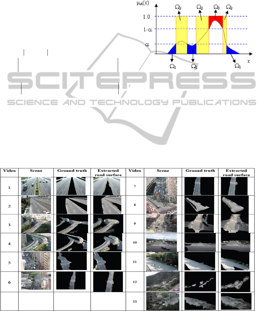
referred to as the rejected (
1
: ( )
: ( )d
μα
μ
≤
Ω
xx
xx
),
marginal (
2
: ( ) 1
: 1d
αμ α
<<−
Ω⋅
xx
x
), and fully accepted (
3
: ( ) 1
: (1 ( ))d
μα
μ
≥−
Ω−
xx
xx
) regions, can be defined.
Figure 6 shows an example membership function,
from which the Ω
1
, Ω
2
, and Ω
3
, regions associated
with a particular α-cut α are indicated. To condense
uncertainty, it leads to the optimization problem of
finding an α-cut that best balances between the
vagueness (Ω
2
) and clearness (Ω
1
+Ω
3
) of the
membership function, i.e.,
α
*
= arg min
α
Ω
1
+Ω
3
−Ω
2
= arg min
α
μ
x:
μ
(x)≤
α
(x)dx + (1−
μ
x:
μ
(x)≥1−
α
(x))dx − 1⋅
x:
α
<
μ
(x)<1−
α
dx
In the discrete case,
*
() ()1
arg min ( ) (1 ( )) cardinal{ | ( ) 1 }
x
α
μα μ α
αμμ αμα
≤≥−
=+−−<<−
x
xxxx
.
We then select α
*
as the threshold of the
membership grades of image pixels to classify them
into road and non-road points.
The above process repeats for different w values. We
start with w = 0, i.e., the definition of membership
grade μ(
x
) of the image pixel at
x
completely
depends on its chamfer distance D(
x
). Thereafter, w
progressively increases, i.e., increasing the influence
of the image characteristic
a
(
x
) of the pixel. In the
beginning, α-cut decreases as w increases. We
terminate the road location step right before α-cut
becomes increasing. This is because we have
empirically observed that α-cut is closely related to
an error rate of road segmentation we defined.
Figure 6: A shadowed set induced from a fuzzy set.
4
EXPERIMENTAL RESULTS
A number of videos taken under various conditions
of weather, illumination, viewpoint, road type, and
congestion have been employed for experiments.
Videos were acquired using a camcorder that
provides 30 images of size 320 by 240 per second.
No particular specification about the installation of
the camcorder has been imposed. The lengths of
Table 1: Experimental results of demonstrative videos.
AutomaticRoadSegmentationofTrafficImages
473

videos range from 2 to 3 minutes. Our algorithm
written in C++ running on a PC at the rate of 2.5Hz
takes about 30 to 150 seconds to complete the road
segmentation of a video. The processing time
depends on the complexities of both traffic and
scene. Specifically, a slowly moving traffic needs a
longer time to build the GMBS model of the scene.
A scene comprising a large portion of road
surface will take time to locate moving objects for
generating a preliminary road segment. In this study,
we pay more attention on efficacy than efficiency.
Table 1 collects the input data, the intermediate
and final results of some experimental videos. We
refer to these videos as demonstrative videos from
now on. The scenes, from which the videos are
acquired, are depicted in the second column of the
table. The third column shows the background
images generated from the GMBS models of the
scenes. We extract by hand from the background
images the road surfaces for serving as ground truths
displayed in the fourth column. The last two
columns demonstrate the intermediate and final
results of preliminary road segment as well as
extracted road surface, respectively. The landscapes
of the demonstrative videos include freeways
(Videos 1 and 2), expressways (Videos 3 and 4),
thoroughfares (Videos 5 and 6), streets (Videos 7
and 8), intersections (Videos 9 and 13), suburban
road (Video 10), campus road (Video 11), and
mountain road (Video 12). In addition to distinct
road types, the demonstrative videos have been
involved different conditions of illumination
(daylight, sunshine and shadow), weather (sunny,
cloudy and rainy days), congestion (rush and off-
peak hours), and viewing direction.
To evaluate the performance of the proposed road
segmentation method, we define the error rate ε of
road segmentation as follows. The symbols N, N
g
,
N
e
, n
g
, and n
e
, they specify the numbers of pixels of
the road image, the ground truth, the extracted road
surface, the extracted road surface in and not in the
ground truth, respectively. Accordingly, the number
of misclassified pixels that are road pixels (i.e., false
negatives) is N
g
-n
g
and the number of misclassified
pixels that are not road pixels (i.e., false positives) is
N
e
-n
g
. The total number of misclassified pixels is
hence
()() 2
gg eg g e g
Nn Nn NN n−+ −=+−
. We
normalize this number with the size N of the road
image to define error rate
2
ge g
NN n
N
ε
+−
=
.
In the road location step, parameter w plays an
important role in defining the membership grades of
image pixels belonging to road surface (Equation 4).
The larger the value, the more significant the image
characteristic and the less influential the chamfer
distance in locating road surfaces. Table 2 shows the
error rates ε of road segmentation of the
demonstrative videos under different w. In this table,
the minimum error rate is marked for each
demonstrative video. The w values corresponding to
the minimum error rates range from 0.2 to 0.35. This
suggests that we may choose w within [.2-s, 0.35+s],
where s is a small value, instead of the entire range
of [, 1]. Although the searching range of w has been
greatly reduced, we still face the issue as to which w
will lead to the minimum error rate of road
segmentation due to the fact that we don’t know the
ground truth during processing.
Recall that for each w an α-cut is determined for
serving as the threshold of the membership degrees
of image pixels belonging to road surfaces. Table 3
shows the α-cuts of the demonstrative videos
decided under different w. In this table, the
minimum α-cuts are marked as well. Surprisingly,
they exactly correspond to the minimum error rates
in Table 2. In other words, minimum α-cuts can be
indicative of minimum error rates. Moreover, the
former are more reliable to identify than the latter. In
our algorithm, the road location step terminates once
the minimum α-cut is observed.
Several factors have impacted on the performance
of our road segmentation. Among these, the viewing
direction of the camcorder may be the most critical
one. In Table 2, the columns corresponding to
Videos 5, 6, and 7 have considerably smaller error
rates than the other columns. As we can see in Table
1, these videos were acquired by the camcorder with
its viewing directions nearly perpendicular to the
road surfaces, or equivalently the tilt angles of the
camcorder close to 90 degrees. Moreover, the tilt
angles of the camcorder increase from Video 5 to 7
and their corresponding minimum error rates
decrease (7.8, 5.5, 4.7). In other words, the larger the
tilt angle of the camcorder the lower the error rate of
road segmentation. Seeing Video 10 in Table 1, it
has the smallest tilt angle of the camcorder among
the thirteen demonstrative videos and has a
relatively high error rate (20.1). This is because
vehicles captured by the camcorder with a small tilt
angle will be more likely to occlude large areas
outside the road.
In Table 2, the columns corresponding to Videos
3 and 4 have considerably larger error rates than the
other columns. Taking look at the experimental
results of these two videos in Table 1, both missed a
large portion of road surface near the top of the road
images. Our algorithm failed to detect moving
objects present in the top rows of images because
VISAPP2015-InternationalConferenceonComputerVisionTheoryandApplications
474
Table 2: Error rates
ε
of road segmentation for the
demonstrative videos under different
w
.
they are too small. Defective preliminary road
segments could result in imperfect road
segmentation. Likewise, if a road area has no vehicle
passing through during constructing the preliminary
road segment, an incomplete road surface may be
extracted. In the suburban road of Video 10, only 6
vehicles passed by during taking the video for about
three minutes. Moreover, none of these vehicles
went through the road area close to the lower left
corner of the road image. The same situation is also
observed in the campus road of Video 11, where
only pedestrians and bicycles are allowed. Both
kinds of the objects are small as well as slow. In
these two cases, longer videos would somewhat
compensate for the drawbacks.
Another video sequence (Video 13) acquired in a
rainy day has relatively large error rates, which are
primarily resulting from the reflections of buildings
on the road surface. The reflections of vehicles
haven’t caused troubles because vehicles are on the
road. The reflections of buildings possess image
characteristics similar to those of the actual
buildings. The lower portions of the buildings
besides the road will be regarded as road areas
because they are close to the road area.
Finally, we compare the method proposed in this
study with that previously reported in (Chung et al.,
2004). Basically, the two methods consist of the
same four major steps. However, the previous
method has several weaknesses. First, the
background model is generated using a
progressively accumulating histogram approach. The
generated background model cannot avoid regarding
such moving objects as flipping leaves
Table 3:
α
-cuts of the demonstrative videos under different
w
.
Table 4: Error rates
ε
of road segmentation for the previous and current methods.
AutomaticRoadSegmentationofTrafficImages
475

and grasses, waving flags and flashing lights as
foreground objects. Second, in the moving vehicle
detection foreground objects are extracted simply
using the background subtraction method. This
method has suffered from illumination changes,
especially shadows, as well as slowly moving
traffics. Third, the morphological process ignores
isolate road regions. This leads to defective
preliminary road segments. Finally, there is no
strategy for dealing with the problem of over-
estimate due to perspective projection of vehicles
moving along the roadside. The above drawbacks
associated with the previous method have been
compensated for in the current method. We have
applied both the previous and current methods to
all the 13 experimental videos. However, the
previous method only worked on six of them (i.e.,
videos 1, 7, 10, 11, 12, and 13). This is probably
because of the associated drawbacks mentioned
above. Table 4 shows the experimental results, in
which except for video 11, the current method has
outperformed the previous one for the rest videos,
especially videos 1 and 12.
5
CONCLUDING REMARKS
AND FUTURE WORK
In this paper, an automatic road segmentation
method was presented. The proposed method is
dedicated to static traffic scenes. Previous
researches have paid more attention on either
dynamic or restricted static scenes. As a matter of
fact, a large number of traffic applications have to
do with static traffic scenes and various conditions
of environment, weather, illumination, viewpoint,
and road type can make the road segmentation of
static traffic scenes challenging too. A number of
video sequences of traffic scenes under different
conditions have been used in our experiments. The
error rates of road segmentation of all experimental
videos were within 25%. In terms of potential
applications, the performance of the proposed road
segmentation method can be acceptable. We will
keep improving the performance of the current
method and develop potential applications in our
future work
REFERENCES
Ndoye, M., Totten V. F., Krogmeier, J. V., and Bullock,
D. M., 2011. Sensing and signal processing for
vehicle re-identification and travel time estimation.
IEEE Trans. on Intelligent Transportation Systems,
12(1), pp. 119-131.
Perez, J., Milanes, V., and Onieva, E., 2011. Cascade
architecture for lateral control in autonomous
vehicles. IEEE Trans. on Intelligent Transportation
Systems, 12(1), pp. 73-82.
Skog, I., and P. Händel, 2009. In-car positioning and
navigation technologies — A Survey. IEEE Trans.
on Intelligent Transportation Systems, 10(3), pp. 4–
21.
Alvarez, J. M., Lopez, A., and Baldrich, R., 2008.
Illuminant-invariant model-based road
segmentation. Proc. of IEEE Intelligent Vehicles
Symp., Eindhoven University of Technology
Eindhoven, The Netherlands.
Chen, Y. Y., & Chen, S. W., 2010. A restricted bus-lane
monitoring system. Proc. of the 23rd IPPR Conf. on
CVGIP, Kaohsiung, Taiwan.
Chung, Y. C., Wang, J. M., Chang, C. L., and Chen, S.
W., 2004. Road segmentation with fuzzy and
shadowed sets. Proc. of Asian Conf. on Computer
Vision, Korea.
Ha, D. M.,
Lee, J. M., and Kim, Y. D., 2004. Neural-
edge-based vehicle detection and traffic parameter
extraction. Image and Vision Computing, 22(11),
pp.899-907.
Alvarez, J. M. and Lopez, A. M., 2011. Road detection
based on illumination invariance. IEEE Trans. on
Intelligent Transportation Systems, 12(1), pp. 184-
193.
Courbon, J., Mezouar, Y., and Martinet, P., 2009.
Autonomous navigation of vehicles from a visual
memory using a generic camera model. IEEE Trans.
on Intelligent Transportation Systems, 10(3), pp.
392-402.
Obradovic, D., Lenz, H., and Shupfner, M., 2008.
Fusion of sensor data in siemens car navigation
system,” IEEE Trans. on Vehicular Technology,
Vol. 56, No. 1, pp. 43-50, 2008.
Danescu, R. and Nedevschi, S., 1994. Probabilistic lane
tracking in difficult road scenarios using
stereovision. IEEE Trans. on Intelligent
Transportation Systems, 10(2), pp. 272-282.
Santos, M., Linder, M., Schnitman, L., Nunes, U., and
Oliveria, L., 2013. Learning to segment roads for
traffic analysis in urban images. IEEE Intelligent
Vehicles Symposium, pp. 527-532, Gold Coast, QLD.
Tan, C., Hong, T., Chang, T., and Shneier, M., 2006.
Color model-based real-time learning for road
following. Proc. of the IEEE Conf. on Intelligent
Transportation Systems, Toronto, Canada.
Sha, Y., Zhang, G. Y., and Yang, Y., 2007. A road
detection algorithm by boosting using feature
combination. Proc. of IEEE Intelligent Vehicles
Symposium, Istanbul, Turkey.
Wang, J. M., Chung, Y. C., Lin, S. C., Chang, S. L., and
Chen, S. W., 2004. Vision-based traffic
measurement system. Proc. of IEEE Int’l. Conf. on
Pattern Recognition, Cambridge, United Kingdom.
VISAPP2015-InternationalConferenceonComputerVisionTheoryandApplications
476

Wang, J. M., Chung, Y. C., Lin, S. C., Chang, S. L., and
Chen, S. W., 2004. Vision-based traffic
measurement system. Proc. of IEEE Int’l. Conf. on
Pattern Recognition, Cambridge, United Kingdom.
Ma, B., Lakshmanan, S., and Hero, A. O., 2000.
Simultaneous detection of lane and pavement
boundaries using model-based multisensor fusion,”
IEEE Trans. on Intelligent Transportation Systems,
1(3), pp. 135-147.
Beucher, S. and Bilodeau, M., 1994. Road segmentation
and obstacle detection by a fast watershed
transform. Proc. of the Intelligent Vehicles Symp.,
pp. 296-301.
Bilodeau, M. and Peyrard, R., 1992. Multi-pipeline
architecture for real time road segmentation by
mathematical morphology,” Proc. of the 2nd
Prometheus Workshop on Collision Avoidance, pp.
208-214, Nurtingen, RFA.
Soquet, N., Aubert, D., and Hautiere, N., 2007. Road
segmentation supervised by an extended V-disparity
algorithm for autonomous navigation,” Proc. of
IEEE Intelligent Vehicles Symp., Istanbul, Turkey.
Mackeown, W. P. J., Greenway, P., Thomas, B. T., and
Wright, W. A., 1994. Road recognition with a
neural network. Engineering Applications of
Artificial Intelligence, 7(2), pp. 169-176.
Wang, J. M., Cherng, S., Fuh, C. S., and Chen, S. W.,
2008. Foreground object detection using two
successive images,” IEEE Int’l. Conf. on Advanced
Video and Signal based Surveillance, pp. 301-306.
Paragios, N., 2006, Chapter 9: Curve Propagation, Level
Set Methods and Grouping. Handbook of
Mathematical Models in Computer Vision, Edited
by N. Paragios, Y. Chen, and O. Faugeras, Springer
Science + Business Media Inc., pp. 145-159.
Comaniciu, D., Ramesh, V., and Meer, P., 2003. Kernel-
based object tracking. IEEE Trans. on Pattern
Analysis and Machine Intelligence, 25(5), pp. 564-
577.
Chen, S. W., Chen, C. F., Chen, M. S., Cherng, S., Fang,
C. Y., and Chang, K. E., 1997. Neural-fuzzy
classification for segmentation of remotely sensed
images,” IEEE Trans. on Signal Processing, 45(11),
pp. 2639-2654.
Pedrycz, W., 2009. From fuzzy sets to shadowed sets:
interpretation and computing. Int’l Journal of
Intelligent Systems, 24, pp. 48-61.
Wang, J. M., Chen, S. W., and Fuh, C. S., 2011.
Gaussian mixture of background and shadow
model. Proc. of the IADIS Conf. on Computer
Graphics, Visualization, Computer Vision, and
Image Processing, Rome, Italy.
Fritsch, J., Tobias, K., and Franz, K., 2014. Monocular
road terrain detection by combining visual and
spatial information. IEEE Trans. on Intelligent
Transportation Systems, 15(4), pp. 1586-1596.
AutomaticRoadSegmentationofTrafficImages
477
